How to Filter in Excel

---

Have you ever wanted to temporarily display only certain data from a larger dataset without deleting the rest? There are a couple of options to do this, including:

• Manually hiding rows or columns
• Using auto filters
• Using advanced filters
• Using the Excel FILTER function

In this piece, we’ll focus on the filter-based methods. Here’s how to filter in Excel.

---

---

Auto filters

To create a simple auto filter:

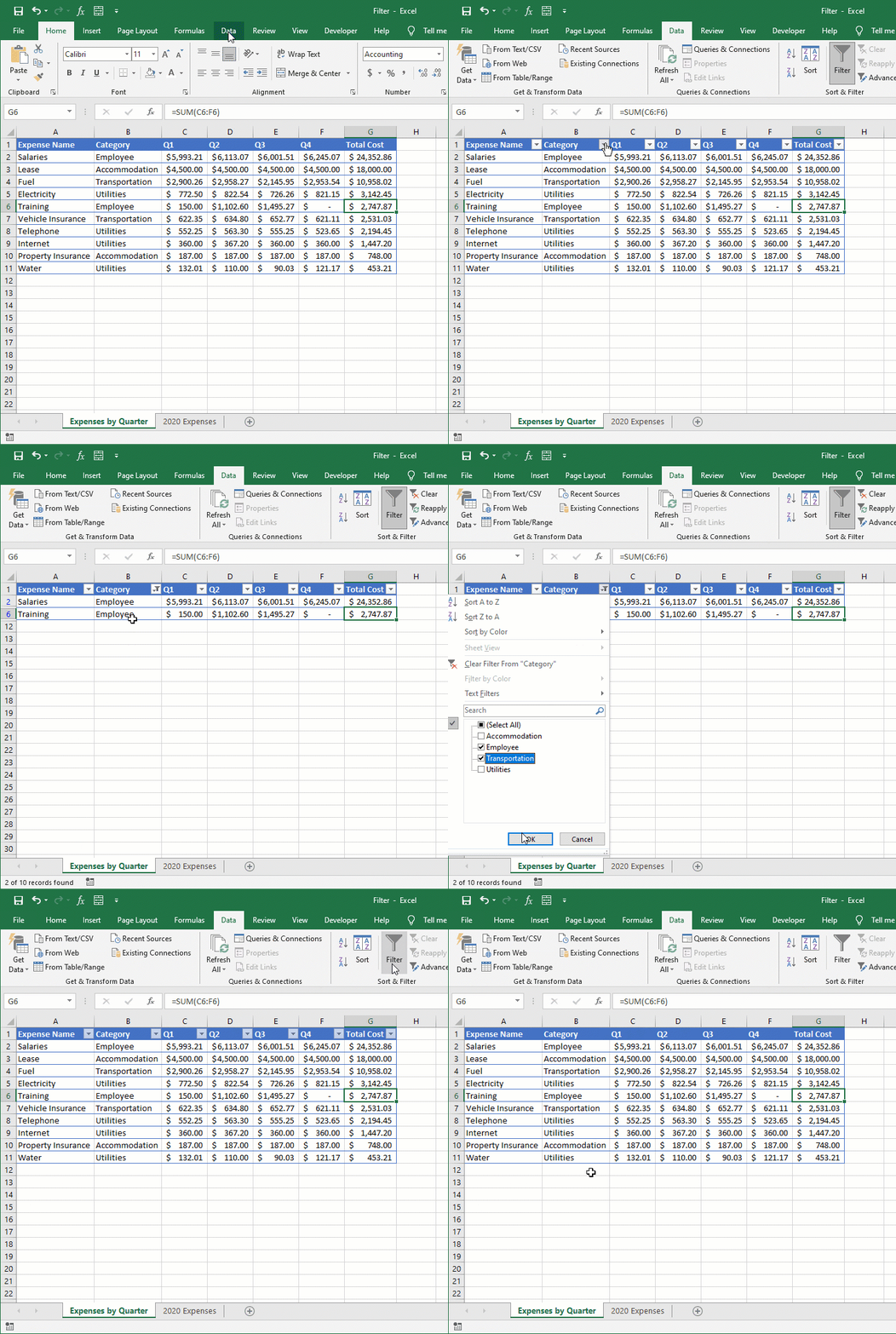
1. Click anywhere within the dataset that you want to create a filter for.
2. Click on the “Filter” icon on the Sort & Filter command group. Excel will then create a filter arrow in the first row of the dataset. If that’s not where you wanted your filter to be, just highlight the row that you want to treat as your header row and click on the “Filter” icon.
3. Each header row now has a dropdown menu that includes a list of unique values that you can choose to filter your data by. Any box that’s unchecked will be filtered out of your display.
4. To clear a filter and redisplay all the data, go back to the filter dropdown and select all categories. Or just deselect the filter icon on the Excel ribbon.

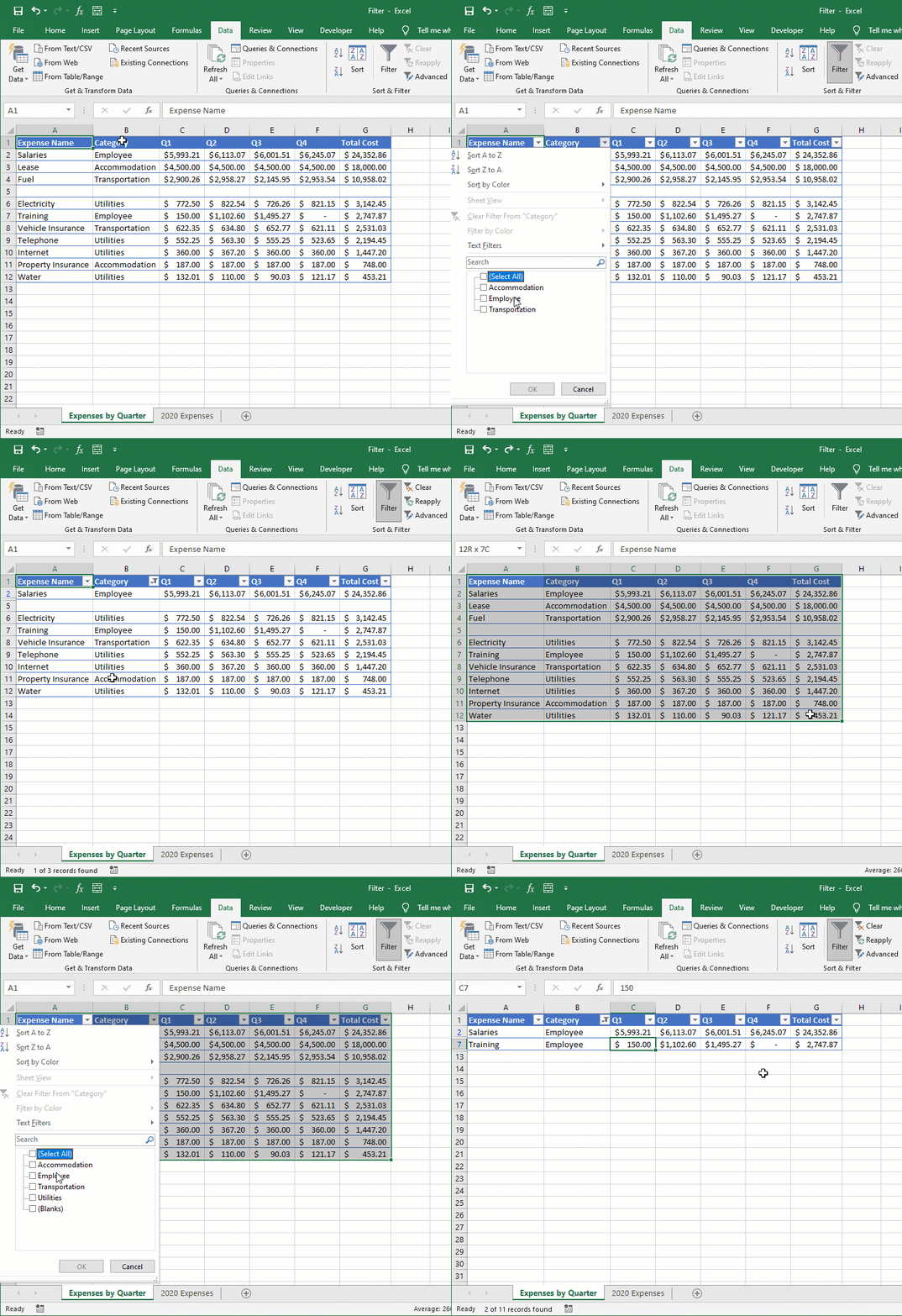
Note that if you have blank rows in your dataset, Excel will assume that your dataset ends just before the blank row. 

If you want your filter to include data above or below your blank rows, then manually highlight the entire dataset — blanks and all, when creating your filter — and it will include the data below your blank rows too.

Applying search and number or text filters

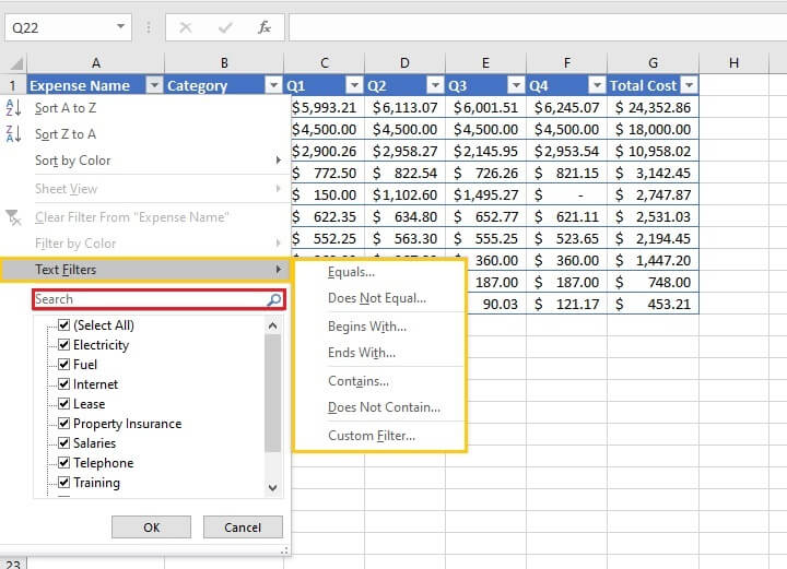
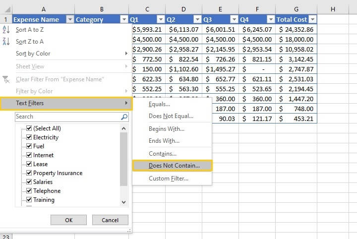
The auto filter dropdown also allows options such as Search and other Advanced or Custom filter fields.

Searching is a convenient alternative to checking or unchecking data from the list and can be used on fragments to extract values that are not identical, but that have some characters in common. 

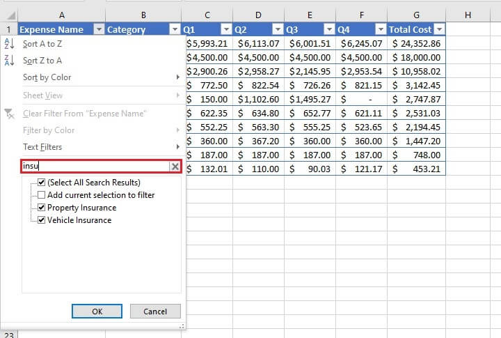
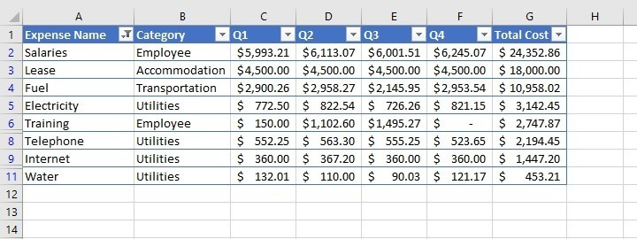
For example, we may want to look at the Insurance expenses. Since there is Property Insurance and Vehicle Insurance, we could scroll down and check both boxes, or we could just type the first few letters of the word Insurance. 

The search results will appear automatically, with the boxes checked. Click OK and the results are displayed.

You can use text filters to display more specific information. This includes cells that contain a certain number of characters or data that does not contain a word you specify. For example, we can go to Text Filters and filter out rows that do not contain the word Insurance.

The Custom AutoFilter window appears. There, you would enter the word insurance.

The results now filter out values that include the word Insurance in column A.

Filter using Excel tables

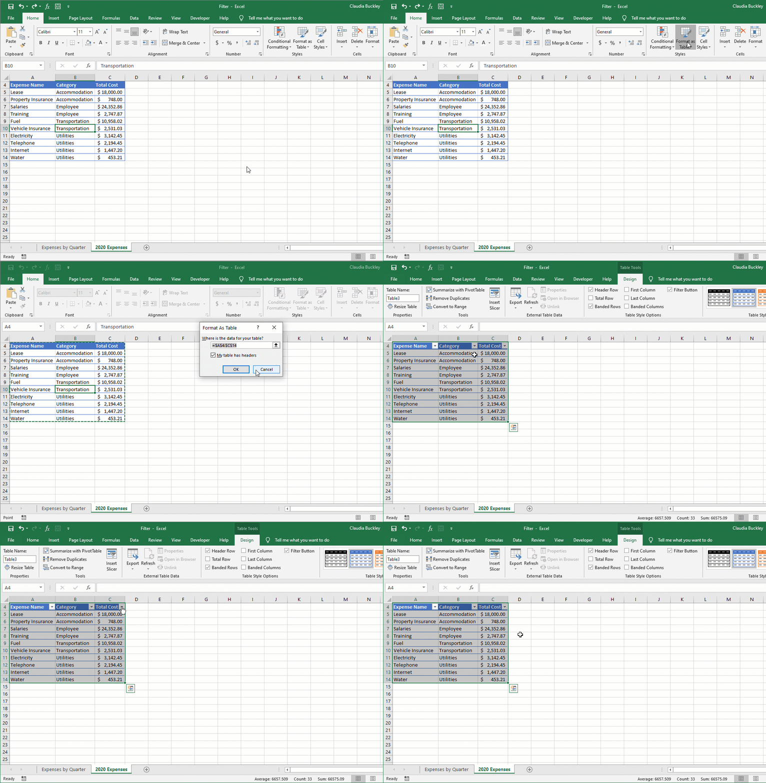
Excel-created tables are automatically created with filter dropdowns, offering the same options referred to above.

Filter using advanced criteria

Excel’s Advanced filter feature also allows you to specify which fields you’d like to include or exclude from your display. It goes a step further by allowing you to display cells that satisfy one criterion OR another, known as OR logic.

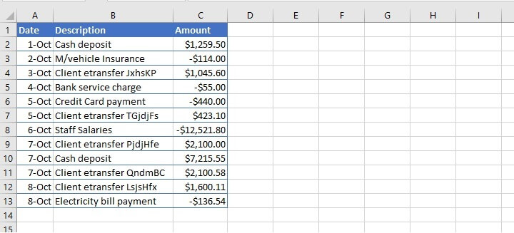
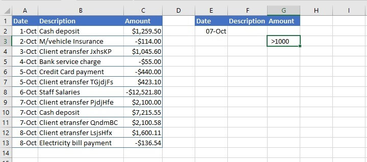
The following example shows banking transactions from October 1 to 8.

Filter with multiple criteria (OR logic)

If we wanted to get all the records that took place either on October 7 or were greater than $1000, then an auto-filter cannot do that. Each criterion is found in a different field and there are some rows that satisfy one criterion but not the other. 

Therefore, filtering out non-October 7 records will remove some records where column C is greater than $1000. So let’s set up an advanced filter.

Our filter concerns two columns: Date and Amount. The best practice is to replicate all headings by copying them and placing them somewhere on the worksheet.

Here’s how to do it:

In the Date column, we’re looking for records with the date October 7, so that date is entered below the Date heading, in column E2. 

The second filter condition refers to the Amount column. Since values may or may not satisfy both conditions, the second criterion should not be placed in the same row as the previous condition. In our example, we’ll place it in cell G3.

To apply these filter conditions:

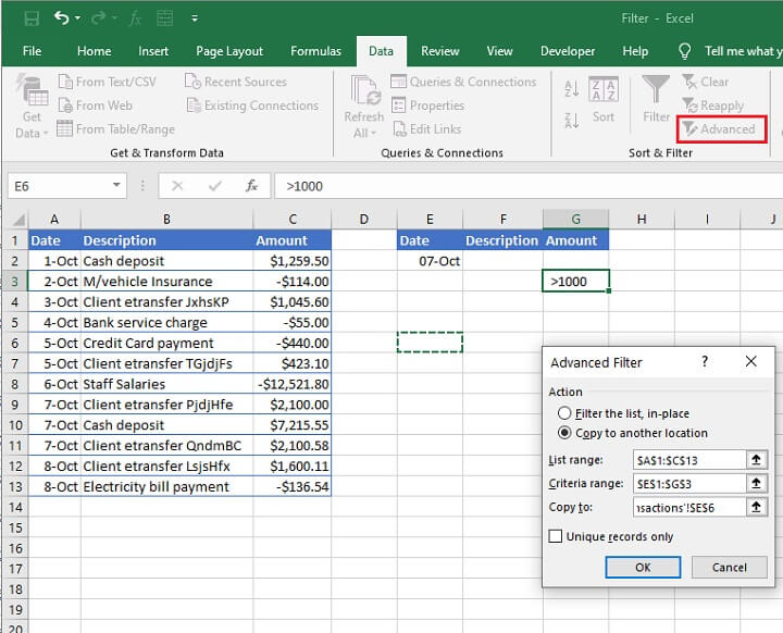
1. Go to the Data tab and click the Advanced filter icon.
2. Choose to either filter the list in place, or copy to another location (within this same worksheet).
3. For ‘List Range’ select the list to be filtered, including column headers.
4. Select the criteria range, i.e., the column name and criteria entered in E1 to G3.
5. If ‘Copy to another location’ was selected, click on the cell where you want the filtered list to appear, in the 'Copy to' field.
6. Click OK.

The filtered list will begin in cell E6, as stated in the ‘Copy to’ field (see below).

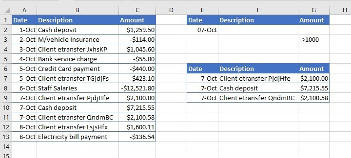
Filter with multiple criteria (AND logic) using wildcards

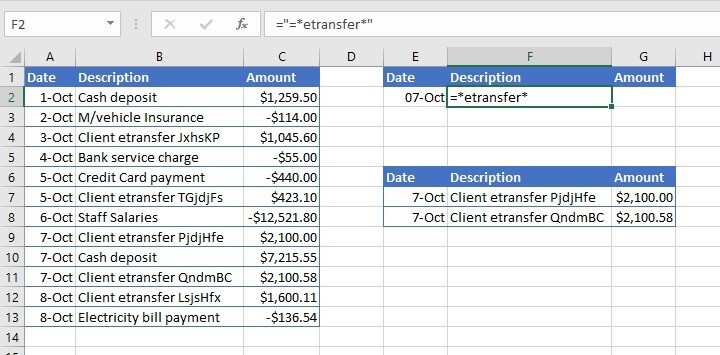
For AND logic where rows should satisfy all stated criteria, conditions should be placed in the same row.

To display transactions made on October 7 which included “etransfer” as part of the description, we would make use of wildcards in that field.

="=*etransfer*"

Asterisks before and after the word “etransfer” search for that word with any number of characters before or after the word.

One drawback with advanced filters is that the filter isn’t dynamic, meaning that it has to be reapplied if you adjust your criteria.

Another limitation is that while your advanced filter can be in a different location on the worksheet, it must be on the same worksheet as the original dataset.

FILTER function

There are other ways to extract specific data from a dataset. With Microsoft 365, we can now use the FILTER function, which, unlike the advanced filter criteria functionality, is dynamic. That means it updates automatically when your data changes, and does allow you to extract data to another worksheet. 

If you don't have Office 365, you can access the FILTER function through Excel on the Web.

The FILTER function syntax is:

=FILTER(array,include,[if_empty])

• Array: the array, or range to filter.
• Include: an array the same height or width as array.
• If_empty: the value to return if the filter returns nothing (optional).

In the example below, we can extract the entries in the “Employee” category with the entry:

=FILTER(A2:C11,B2:B11="Employee","")

An explanation of the formula above is as follows:

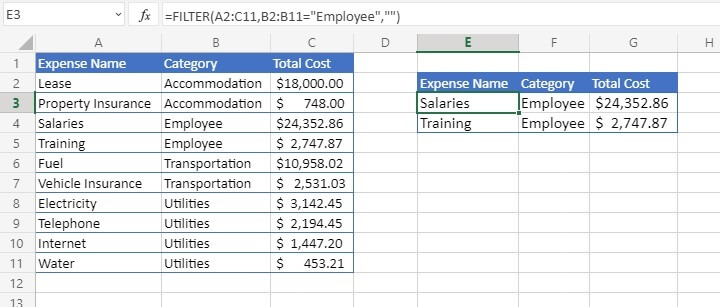
• A2:C11 - the entire original dataset. 
• B2:B11="Employee" - look in range B2 to B11 for the text Employee.
• “” - display nothing if no rows meet the criterion.

It is more common for the filter criterion to be entered in a separate cell (e.g., F1) and use a cell reference instead of hardcoding the value directly in the formula:

=FILTER(A2:C11,B2:B11=F1,"")

Here is an example of alternative text if the FILTER function returns no valid results:

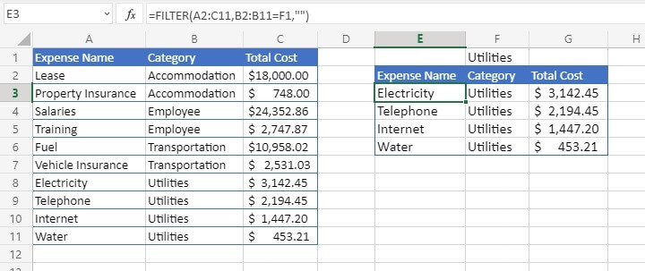
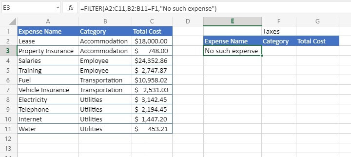
=FILTER(A2:C11,B2:B11=F1,"No such expense")

Notes on the FILTER function: 

• Text values are enclosed by double quotes and are not case-sensitive.
• Cell reference criteria are not enclosed by double quotes.
• The FILTER function will return an array. This will spill if it's the final result of a formula. This means that Excel will dynamically create the appropriately sized array range when you press ENTER. 
• If there aren’t enough empty cells to return all the results, Excel will return a #SPILL! error.
• If your dataset has the potential of returning an empty value, then use the 3rd argument ([if_empty]). Otherwise, a #CALC! error will result, as Excel does not currently support empty arrays.
• If any value of the ‘include’ argument is an error (#N/A, #VALUE, etc.) or cannot be converted to a Boolean expression, the FILTER function will return an error.  
• If the source data is in another workbook, both workbooks must be open. Otherwise, Excel will return a REF! error.

Summary

That’s how to filter in Excel. There is no shortage of Excel’s capabilities to extract exactly what we need by using one of its filter features. You just learned a few of the ways we can apply simple and complex filters to different types of data. 

How about checking out the full Microsoft Excel course to become the Excel pro you always wanted to be? Or you can start with some basics in Excel by trying the free Excel in an Hour course first.

Learn Excel for free

Start learning formulas, functions, and time-saving hacks today with this free course!

Start free course