VLOOKUP With Multiple Criteria or Multiple Results in Excel

VLOOKUP is one of the most widely used functions in Excel, known for its ability to look up values in a database or table. You may already be aware that it has basically been replaced by XLOOKUP, but if you want to lookup multiple values in Excel, we're here to help you navigate this (occasionally tricky) task.

It might be that you want to display results matching any of several criteria (OR logic), or perhaps you only want to see results that match all criteria (AND logic). You might even want to take it a step further by returning multiple match results, instead of just the first matching result, which is all VLOOKUP can do. 

Multiple options

There are several possible approaches you could take, all of which are summarized in the chart below.  

Method	Lookup Multiple Criteria (using OR logic)	Lookup Multiple Criteria (using AND logic)	Return Multiple Results
FILTER function	Y	Y	Y
Advanced Filter	Y	Y	Y
Auto Filter	Only criteria within the same column	Y	Y
XLOOKUP	N	Y	No, but can spill from contiguous rows and columns
VLOOKUP & Helper	N	Y	N
VLOOKUP MATCH	N	Max 2 criteria; data with matrix layout	N
INDEX MATCH MATCH	N	Max 2 criteria; data with matrix layout	N

As you can see, performing a VLOOKUP with multiple criteria may not even include VLOOKUP at all! We’ll explore each of these methods in the examples below.

FILTER function

When it comes to the best option to achieve this function, the hands-down winner of this competition is the FILTER function. FILTER was specifically created to match multiple criteria in an array and return all results that match those criteria. Best of all, it is dynamic, so the results update when the criteria change. Its ability to spill multiple values is native to the function and does not require any special maneuvers. 

Return multiple results

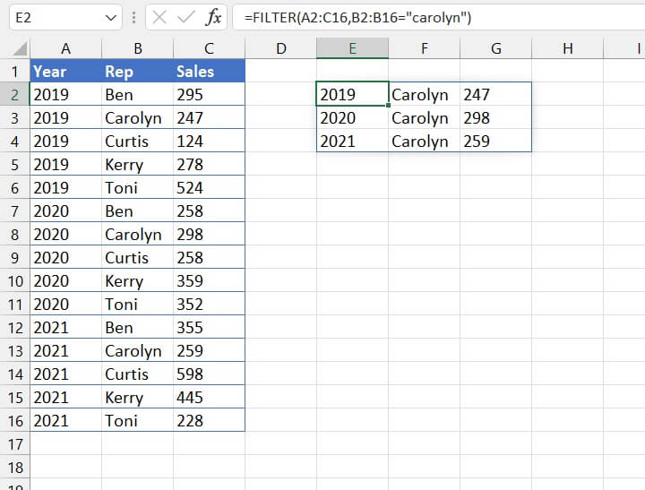
• For the array argument, input the range of cells from which the results should be returned.
• For the include argument, select the row or column to be evaluated and pair that with the relevant logical argument.

=FILTER(A2:C16, B2:B16="carolyn")

Lookup multiple values

• To lookup multiple criteria using OR logic with the FILTER function, modify the syntax of your formula so that the include argument consists of each criterion enclosed in parentheses and separated by a plus sign.

The standard FILTER syntax is:

=FILTER(array, include, [if_empty])

which translates to

=FILTER(B2:C16,(B2:B16="ben")+(B2:B16="toni")+(B2:B16="curtis"))

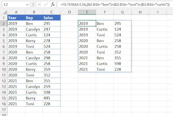
The formula above looks for any instances where column B matches either “Ben”, “Toni”, or “Carolyn” and returns all the results.

• To lookup multiple criteria using AND logic with the FILTER function, modify the syntax of your formula so that the include argument consists of each criterion enclosed in parentheses and separated by an asterisk.

The standard FILTER syntax:

=FILTER(array, include, [if_empty])

is applied as follows:

=FILTER(B2:C16,(A2:A16=2020)*(B2:B16="carolyn"))

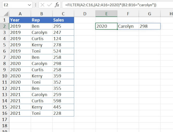
The above formula looks for instances where the value in column A is equal to 2020, AND the same row carries the value “Carolyn” in column B.

Notes about the FILTER function:

• The FILTER function is not available for versions prior to Microsoft 365. However, it can be used in Excel for the Web.
• If there aren’t enough empty cells to return all the results, Excel will return a #SPILL! error.
• To control the way the results are displayed, consider combining FILTER with the SORT function.

Advanced Filter

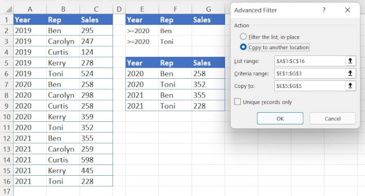
Like the FILTER function, advanced filters also allow you to match multiple criteria in Excel and return multiple results. The main thing to remember when entering criteria with this method is that for AND (must satisfy all) conditions, the criteria should be placed in the same row, but for OR (satisfy any) conditions, they should be placed in separate rows.

The following filter looks for any records belonging to Ben or Toni and extracts them to the stated location.

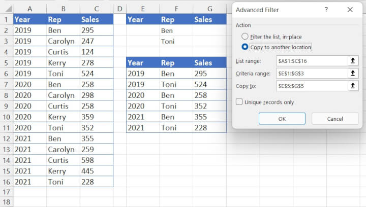
This next filter extracts records where the year is greater than or equal to 2020 for Ben or Toni. 

Notes:

• The Advanced command can be found on the Data tab of the Excel ribbon, within the Sort & Filter command group.
• The biggest drawback with advanced filters is that they are static, so when the source data changes, the list is not updated. The process must be repeated.
• For more ways to use complex criteria with advanced filters, check out this resource from the folks at Microsoft.

Auto Filter

If you want Excel to return multiple results for a lookup value, you might need to look no further than the humble filter. Filters can both lookup multiple criteria and return multiple results.

In the scenario below, we can easily choose to display all sales from a particular sales rep.

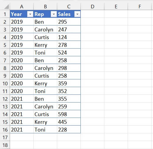
• Click anywhere in the data set. Go to the Data tab and click the Filter icon.
• Go to the category you want to filter by (in this case, “Name”) and choose the filter criteria. You can lookup by value, color, or logic (equal to, greater than, etc.)
• We would remove checkmarks from the names we don’t want to see.

This will return all records for that employee, as shown below.

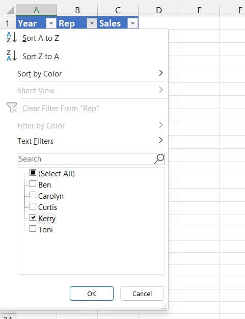
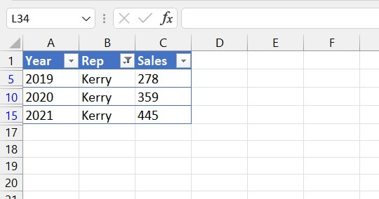
Auto-filters can also match multiple criteria, but in a limited way. So when we select multiple reps, all their records would be displayed. 

However, since the filtering process hides records that do not satisfy the criteria, auto-filters cannot lookup multiple criteria from different categories using OR logic (return records that satisfy any of the stated criteria). 

So if we applied auto-filters to find records for the year “2021” and then another filter for sales less than 200, we would get no results because all sales in 2021 were greater than 200. Therefore, filtering across multiple categories uses AND logic (must satisfy all criteria).

Note:

• Auto filters are only designed to filter out rows, not columns.

XLOOKUP

XLOOKUP has certain built-in advantages over VLOOKUP. One such advantage is that it enables Excel to look up multiple criteria without the need for a helper column. The standard XLOOKUP syntax (without optional arguments) is:

=XLOOKUP(lookup_value, lookup_array, return_array)

• Use the ampersand operator to combine multiple lookup values into a single argument.
• Use the ampersand operator to point to each respective lookup array.

=XLOOKUP(F2&F3, A2:A16&B2:B16, C2:C16)

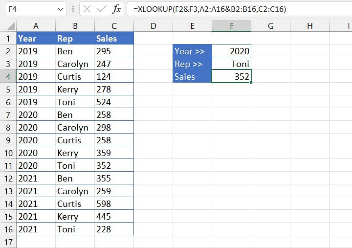
Whenever the stated criteria appear in the same position number of their respective arrays, XLOOKUP returns the contents of that cell.

Return a spilled range

The return array may also be entered as a two-dimensional array so that XLOOKUP spills the contents of the adjoining cells in the matching column or row.

=XLOOKUP(F2&F3,A2:A16&B2:B16,A2:C16)

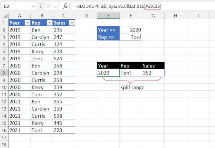
Notes:

• XLOOKUP is not available for versions prior to Microsoft 365. However, it can be used in Excel for the Web.
• This method may be used to combine any number of criteria.
• VLOOKUP works best for unique values within a data set. It can spill a range of cells but cannot return multiple matches.​​

---

---

VLOOKUP with a helper column

If your data set is not complicated, you can use a little creativity to perform a VLOOKUP with multiple criteria, for example:

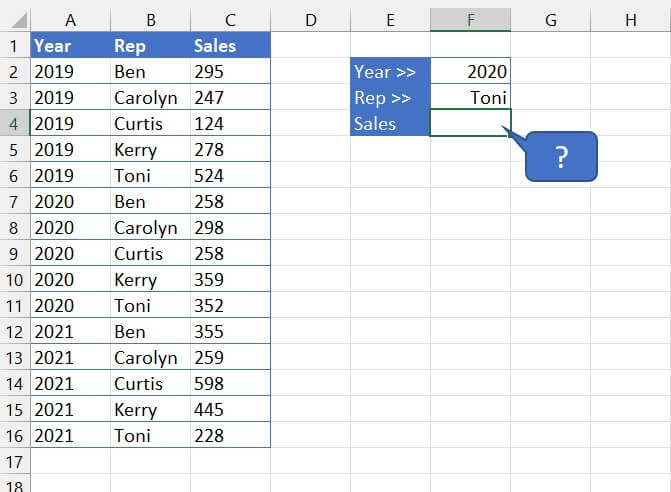
• In a helper column, use the ampersand (&), also known as the concatenation operator, to turn multiple values into a single string. 
• Place the helper column so that it appears anywhere to the left of the column containing the values you want to return. 
• In your VLOOKUP formula, use the ampersand operator to combine multiple lookup values.
• The helper column must be the first column of the table_array.

=VLOOKUP(G2&G3,C2:D16,2,FALSE)

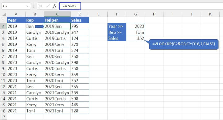
Notes:

• VLOOKUP looks for the combination and uses the first matching value to return a result.
• This method may be used to combine any number of criteria.
• Take care when inserting columns into source data, as doing so may affect dependent formulas elsewhere.

VLOOKUP MATCH

You may already be familiar with the INDEX MATCH vs. VLOOKUP debate, and know that there will be times when it’s better to use INDEX MATCH. Most people though, prefer VLOOKUP simply because it is usually easier to use. 

If your data has a two-dimensional, matrix layout and you want to perform a VLOOKUP on multiple criteria, you might be a bit stumped.

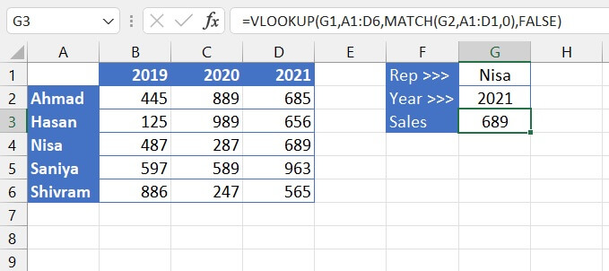
Since VLOOKUP is designed to do a vertical lookup, we just need to insert a MATCH formula in place of the col_index_num argument. Doing so will locate the lookup value on the horizontal axis and return its position (or column) number.

• The lookup_value for VLOOKUP should be for the values that are listed vertically. In this case, it will be cell G1.
• The table_array will be the entire data set, A1:D6.
• For the column_index_num argument, nest the MATCH function so that the column number updates dynamically depending on the value entered in G2.

=VLOOKUP(G1,A1:D6,MATCH(G2,A1:D1,0),FALSE)

Notes:

• Use this method when you want to perform a two-way lookup on a two-dimensional array.
• This method is used for a maximum of two criteria.
• VLOOKUP MATCH uses the first matching value to return a result.

INDEX MATCH MATCH

This method is almost identical to the VLOOKUP MATCH approach above. The usual INDEX MATCH combo uses the syntax

=INDEX(array,(MATCH(lookup_value,header_range*,0),column_num)

or

=INDEX(array,row_num,(MATCH(lookup_value,column_array*,0))

*argument name for explanatory purposes only

In each case, the formula assumes that there is only one lookup value and that either its row or column number is unknown, but not both. 

In the scenario below, we want to look up two values whereby their position on the vertical and horizontal axes could fall anywhere within the array. This makes it a challenge to use INDEX MATCH with multiple criteria.

The solution is simply to plug a second MATCH formula into the sequence.

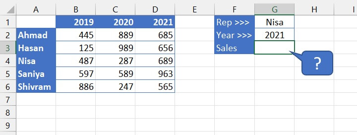
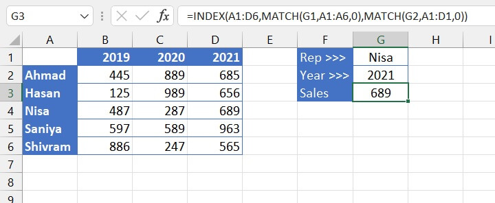
• For the row_num argument, insert the MATCH formula using the value that will fall on the vertical axis.
• For the column_num argument, insert the MATCH formula using the value that will fall on the horizontal axis.

=INDEX(A1:D6,MATCH(G1,A1:A6,0),MATCH(G2,A1:D1,0))

Notes:

• INDEX MATCH MATCH uses the first matching value to return a result.
• This method can be used for a maximum of two criteria.

Don't stop now!

Like what you just learned? We have lots more free Excel tips in our resource library. Better yet, check out our popular Excel Basic and Advanced course today and learn how you can become a certified Excel superhero! 

Ready to become a certified Excel ninja?

Start learning for free with GoSkills courses

Start free trial