How to Merge Cells and Split Cells in Excel

---

Excel is good for handling data, but there are times when you want to combine cells into one value or to split a string to make the data more manageable. 

Excel has several features which give us the ability to merge and split cells in multiple ways. Here’s how to merge cells in Excel and how to split cells in Excel.

How to merge two or more cells

Every now and then in Excel, you'll need to merge two or more cells in a range. One example may be in the case where a dataset is spread across several columns, and for the sake of presentation, you may want to merge the cells containing the heading or title of that dataset to make them behave like one cell.

At other times, ‘merging a cell’ may mean extracting and actually combining data that are located across several rows or columns and placing them in another row or column.

Let’s talk about how to do both.

---

---

Merge & Center

A quick and common way to merge cells is to use the Merge & Center command in the Home tab. 

Simply highlight all the cells to be merged, then click the Merge & Center icon.

In the example above, cells A1 and B1 were highlighted then the Merge & Center command was selected. The result is that both cells now behave like a single cell, which is given center alignment. The cell alignment may be changed if desired.

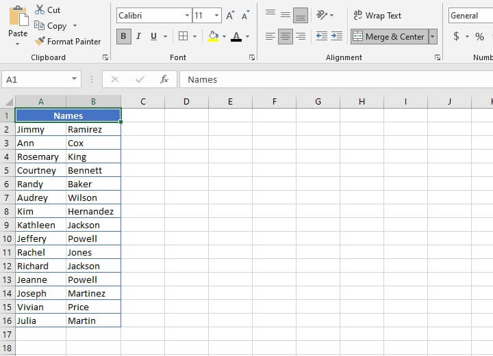
Limitations of Merge & Center

• It should be noted that Merge & Center is only a formatting command. Data from multiple cells will not be combined when using Merge & Center.

• If there is data in the cells being merged, Excel will only keep what is in the upper leftmost cell. If you attempt to merge cells where data is in any other cell, Excel will return the error message, “Merging cells only keeps the upper-left value and discards other values.” In other words, you will lose any data that isn’t in the first cell.

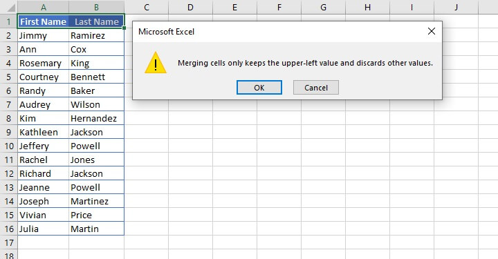
• Another limitation when you use the Merge & Center option to merge cells is that it also prevents you from being able to sort any data that is located in cells that have been merged. 
• Yet another issue is that highlighting a column that contains merged cells will result in highlighting all the columns spanning the merged cells, not just the column that was selected.

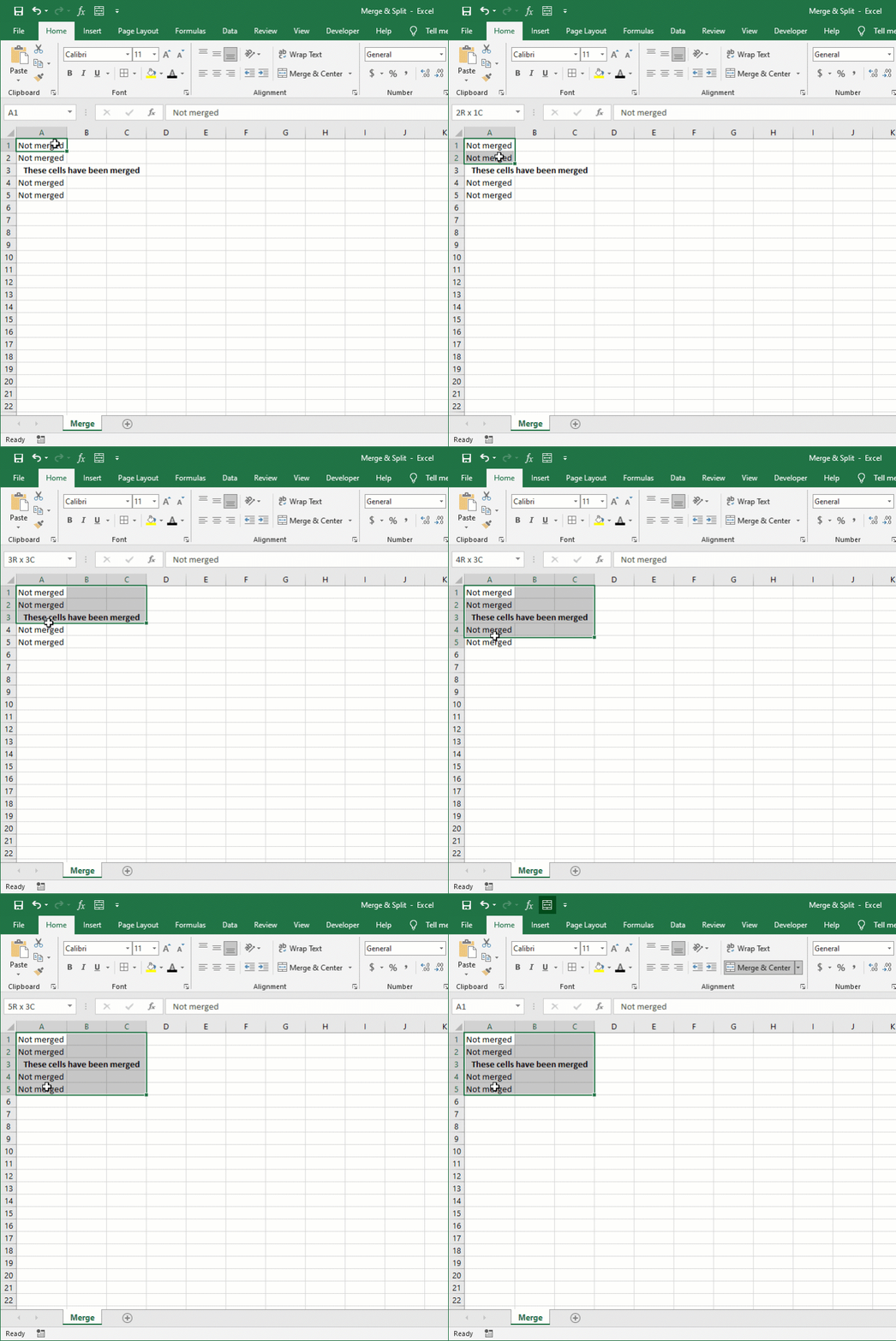
Alternative to Merge & Center

If you want to merge cells in different columns in a single row, the Center Across Selection offers a good solution. The command is not as easy to find in Excel as the Merge & Center option, which is a pity, but it does allow sorting and highlighting without any issues.

To use Center Across Selection:

• Select the cells that you want to merge.
• Press Control + 1 to open the Format Cells dialog box.
• In the Alignment tab, from the Horizontal drop-down, select Center Across Selection.

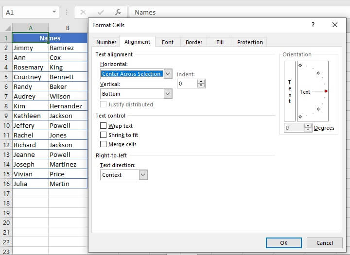
• Click OK.

Using this method will display the text as though it has been merged and centered, but each cell can still be selected one by one, separate from each other. Cells can also be sorted and highlighted as usual.

If data is in any cell other than the upper leftmost cell, there will be no loss of data. Instead, cells will appear as normal, as though they have not been merged.

Combine text from two or more cells into one cell

There are other times when “merging cells” refers to combining the actual data that is in multiple cells into one cell.

This can be accomplished through concatenation.

Three simple methods to concatenate or join values in Excel are shown below. They are:

1. Using the concatenation operator (& symbol)
2. Using the CONCAT function
3. Using the TEXTJOIN function

Each of these methods is designed to join two or more text strings into one string.

Merge cells using the concatenation operator

Using the ampersand (&) symbol between values will join them in a string.

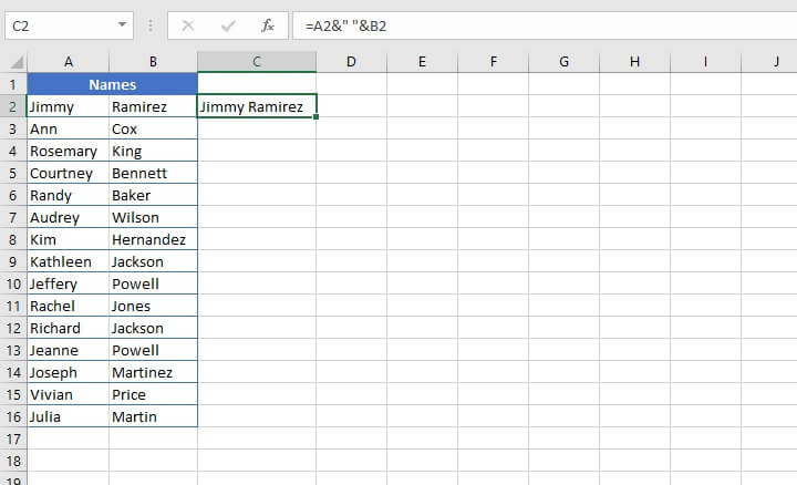
For example, in the dataset below, let’s say we want to have the full name of each individual shown in a single column, column C. Using the & symbol as a concatenation operator is a popular choice because knowledge of function formats is not required although this method is, technically speaking, a formula.

As with all Excel formulas, we would begin with an equal sign. Next, separate each value with the & symbol. Since a space is also likely desired between the first and last names, we would also enter a space within double-quotes. 

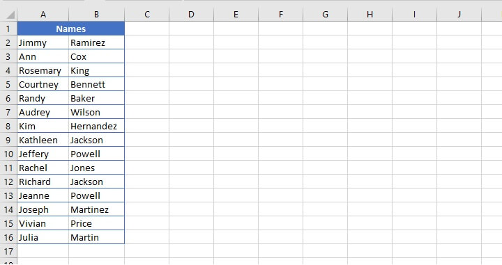
=A2&" "&B2

Merge cells using CONCAT function

The CONCAT function allows the selection of a range and is therefore potentially quicker than using the & symbol, especially when no additional characters are required between the cell values being joined.

This would work well in the case of the dataset below:

The syntax of the CONCAT function is:

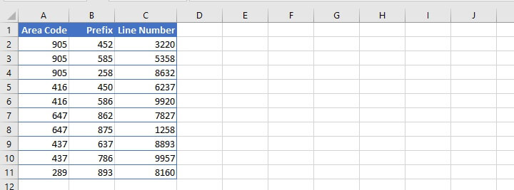
=CONCAT(text1, [text2]...)

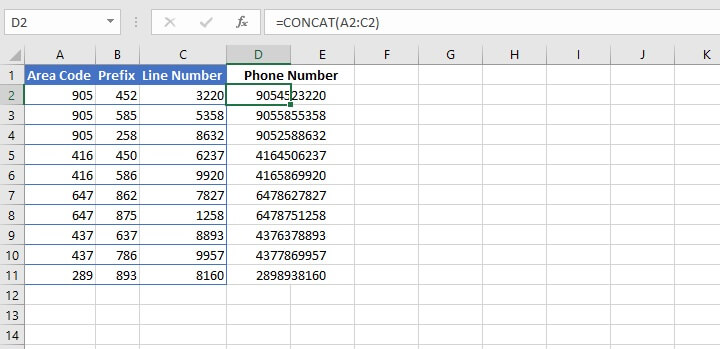
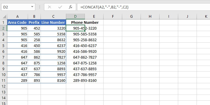
We can merge the contents of cells A2 to C2 in cell D2 with the entry:

=CONCAT(A2:C2)

If additional characters are required between cell values, these would be entered within double quotes and separated by commas as is usually the case with function arguments.

=CONCAT(A2, “-”, B2, “-”,C2)

Merge cells using TEXTJOIN function

TEXTJOIN can be considered an improvement in the efficiency of CONCAT since it allows repetitive delimiters (characters between values) to be entered once.

The syntax of TEXTJOIN is:

TEXTJOIN(delimiter, ignore_empty, text1, [text2], …)

The ignore_empty argument is required and is a setting that tells Excel what to do if empty cells occur within the range. If set to TRUE, empty cells are ignored. If set to FALSE, the delimiter is returned nonetheless, resulting in consecutive delimiters with no values in-between.

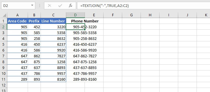
We can insert dashes between each cell value with the entry:

=TEXTJOIN("-",TRUE,A2:C2)

Click here to learn more about using formulas to merge cells in Excel.

Split one cell into two or more

For those times when you’d like to split a single cell with data into two or more columns, the Text to Columns command may be just the thing you need.

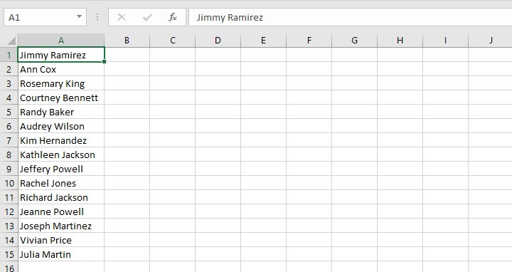
For example, let’s say we have the following name list, and we want the names to be split across two columns.

Method 1 - Split cell using Text to Columns command

We would do the following:

• Select the cells which contain the text to be split (A1:A15).
• Click on the Data tab.
• In the ‘Data Tools’ group, click the ‘Text to Columns’ command.

• In the Convert Text to Columns Wizard:
  • Step 1 of 3: Select the Delimited radio button. This allows you to use a specified character to determine where the column break(s) should be. 

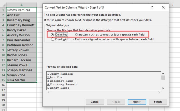
• Click Next.
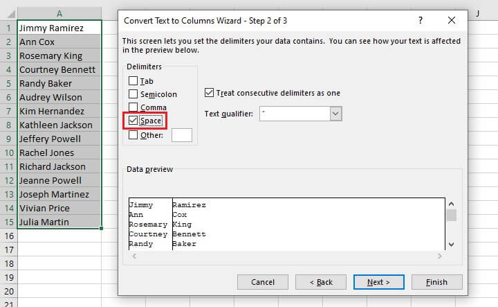
• Step 2 of 3: Select Space as your delimiter. A preview of what your data will look like is shown in the Data Preview section at the bottom of the dialog box.

• Click Next.
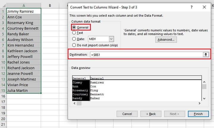
• Step 3 of 3: The Column data format section allows you to specify the format of each column as General, Text, or Date format. If there is a particular column that you do not want to be imported, select it in the Data preview pane and click ‘Do not import column (skip)’ in the Column data format section. The destination field tells Excel where to place the first cell in your new dataset. The default will always be the first cell of your original data. This, of course, means that your original data will be replaced. If you want to be able to compare your new dataset with the original, choose another cell as your destination. In this case, we will choose cell B1.

• Click Finish.

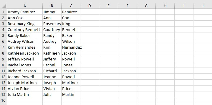
The result is that the text in column A has been split across columns B and C, using the spaces as delimiters.

Method 2 - Split cell using Flash Fill command

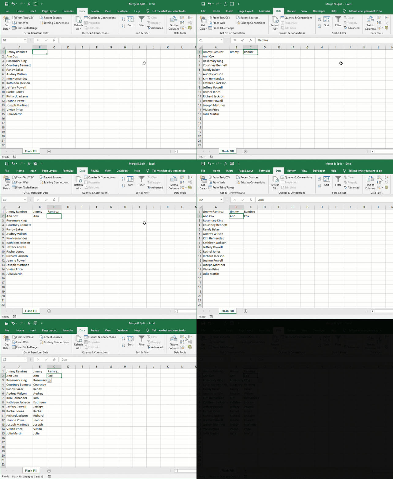
With Flash Fill, you can teach Excel what you want your data to look like by entering the first two or three rows with the data in the desired format.

Next, click on the last value you entered, then click the Flash Fill icon from the Data tab in the Data Tools command group.

Repeat for each column, and voila! Your one-column data has been split across two columns.

Method 3 - Split cell using a formula

Finally, you can also use the LEFT, MID, and RIGHT formulas to break up the values in cells according to their position within the string.

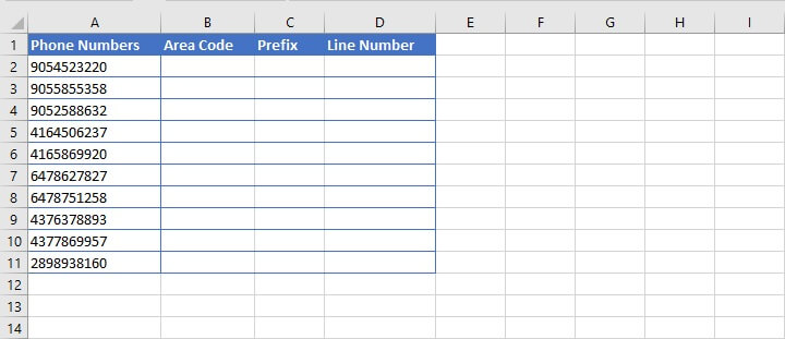
For example, let us assume that we have the following dataset containing telephone numbers, which we would like to split into three separate columns as follows:

• The area code, consisting of the first three numbers. 
• The prefix, consisting of the next three numbers. 
• The line number, consisting of the final four numbers. 

The syntax of the LEFT function is:

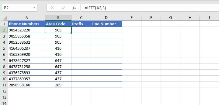
=LEFT(text, [num_chars])

Num_chars is the number of characters in text to return, starting with the leftmost character. If omitted, only the leftmost character is returned.

=LEFT(A2,3)

This formula asks Excel to extract the three leftmost characters from the string in cell A2.

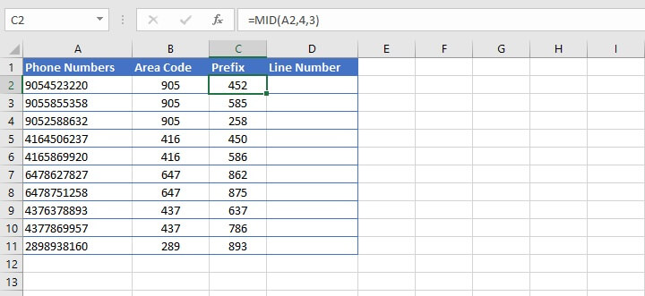
The syntax of the MID function is:

=MID(text, start_num, num_chars)

Start_num is the position number of the first character to be returned, counting from the leftmost character in text.

Num_chars is the number of characters in text to return, starting with the leftmost character. 

=MID(A2,4,3)

This formula asks Excel to extract three characters from the string in cell A2, starting with the fourth character from the left.

The syntax of the RIGHT function is:

=RIGHT(text, [num_chars])

Num_chars is the number of characters in text to return, starting with the rightmost character. If omitted, only the rightmost character is returned.

=RIGHT(A2,4)

This formula asks Excel to extract the four rightmost characters from the string in cell A2.

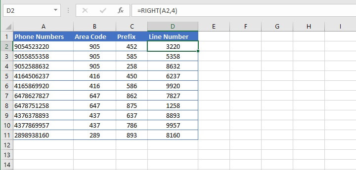
Now we have successfully split the text in one cell into three cells using a formula.

---

Challenge me!

Take this FREE Excel challenge to test out your newly-acquired skills.

---

Learn more

With all these different ways to merge and split cells in Excel, including the data in those cells, you’re bound to find one that suits your needs. Have you found any other methods useful? Join the GoSkills Slack community and share them with us!

You can also check out our course library to learn some other useful techniques in Excel. You can start with our free Excel in an Hour course to cover some basics. Then upgrade your Excel skills with our comprehensive Basic to Advanced Excel course.

Learn Excel for free

Start learning formulas, functions, and time-saving hacks today with this free course!

Start free course