How to Alphabetize in Excel

---

Placing items in alphabetical order is one of the most common ways of organizing data. This is because it uses a standard system (the alphabet) to arrange items, so there is an accepted location for each item on the list.

Since Excel is all about handling and organizing data, it’s no surprise that this is one of the built-in tasks it handles really well.  

Here’s how to alphabetize in Excel.

Alphabetize columns in Excel

Method 1 - Using the A-Z icon

Using the data set below as a sample, we would probably want to alphabetize by last name using Column A.

The absolute quickest way to alphabetize columns in Excel is to use the “A to Z” icon on the Data tab.

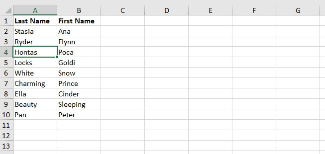
Step 1 - Click on a cell in the column you want to sort by. Notice that A4 is our active cell in the above example.

Step 2 - Go to the Data tab and click this icon:

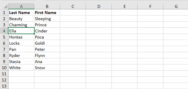
The last names will be sorted alphabetically in ascending order by the column of your active cell.

Of course, you can also see that there is an option to sort in descending order by using the “Z-A” sort icon instead.

---

---

Method 2 - Using the Filter command

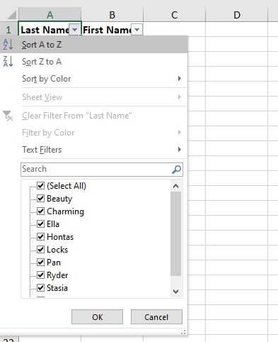
An alternative to the above method is to use the Filter command, also on the Data tab. To do so:

Step 1 - Click on a cell in the column you want to sort by.

Step 2 - Go to the Data tab and click this icon:

Step 3 - Click the dropdown arrow list on the Last Name header, and select the Sort A to Z command from the context menu.

Step 4 - Click OK.

The dataset is sorted with the same results as the previous method and shows a tiny arrow next to the Column A dropdown arrow. If the list had been sorted from Z to A, the arrow would have been shown in the opposite direction.

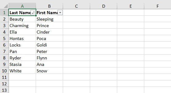
To remove the filter dropdown arrows, click on the Filter icon again.

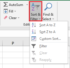
Both the Sort and Filter options are also accessible from the Home tab by using a dropdown menu and selecting their respective icons.

These two “quick-sort” methods work well on this dataset because Excel made the following assumptions:

1. You wanted to sort by columns.
2. Row 1 is a header row and should not be sorted with the list of names.
3. Columns A and B are elements of a single dataset, so rows should be kept together when a column is sorted. 

In this case, these assumptions were all correct, so everything worked out well. Sometimes though, the dataset to be sorted is some variation of the above conditions, so the “A to Z” or “Z to A” icon won’t do.

Sort alphabetically by multiple columns

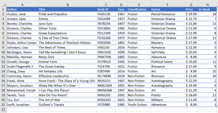
For example, some datasets have several columns with different potential sorting categories, like the database of books in the image below.

Of course, we can sort by any column we want to by using the “A-Z” icon, but this only allows us to sort by one column at a time. If we wanted to sort alphabetically by multiple columns, the “Sort” command is a much better option, as it gives us more options and more control over how our data is sorted.

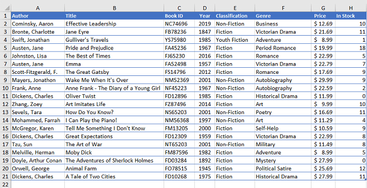
We may want to apply multi-level sorting by first separating books into fiction versus nonfiction, and then alphabetically by the author’s name.

To carry out this task:

1. Click anywhere within the dataset.
2. Go to the Data tab on the ribbon and click on the “Sort” command.

3. Excel automatically detects the dataset to be sorted and displays the Sort dialog box on the screen.

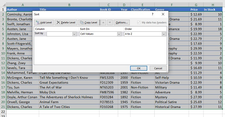
4. Click the “Sort by” dropdown arrow and select the Classification column. The data will be sorted based on the cell values, and in the A-Z order, which is the default.
5. To add a second sorting level, click the “Add Level” button and select the Author column.

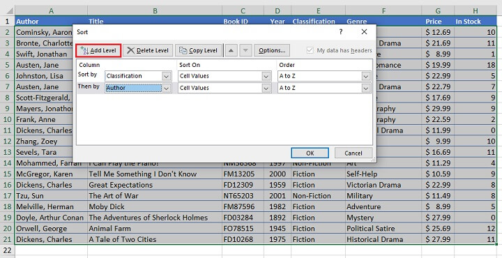
6. Click OK.
7. The data is now reorganized. Fiction books appear at the top of the list, with their authors being listed from A to Z. Non-Fiction books are grouped alphabetically next.

Put rows in alphabetical order

Less often, we may have rows that we want to alphabetize. We can imagine a dataset like the one below, for instance, where we have the number of book copies available by author.

We may want to have this list shown by order of the authors’ names. Using the quick “A-Z” sort method would assume that we want to sort by column, which isn’t the case this time. Using the “Sort” icon instead would give the option to sort by row.

Of special note is that this dataset doesn’t look like most tabular datasets, so Excel may not identify header rows correctly. To make sure that you don’t get any unexpected results, do the following:

1. Highlight the data to be sorted. In this example, we would not highlight the text in Column A since we do not want it shifted when the data gets sorted.

2. Click the “Sort” icon from the Data tab.

3. Uncheck My data has headers.
4. Click Options.
5. Select the “Sort left to right” radio button and click OK.

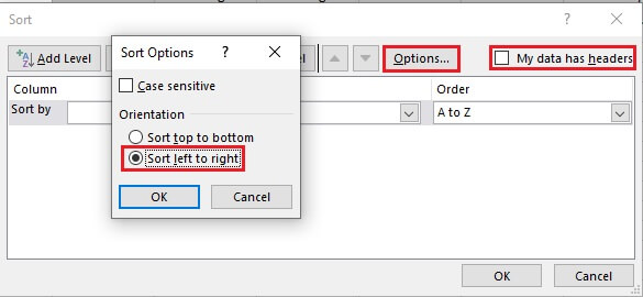
6. From the “Sort by” dropdown list, choose Row 1. Click OK. 

The authors’ names in Row 1 are now sorted alphabetically from left to right.

Unexpected results when sorting alphabetically in Excel

1. Header row gets sorted among data

This happens when Excel doesn't recognize your header row, so it thinks it should be sorted with the data below.

Simply clicking on a single cell and pressing the “A to Z” or “Z to A” icon is a sure way to send yourself into a panic. Instead, if you want to alphabetize by the last name values:

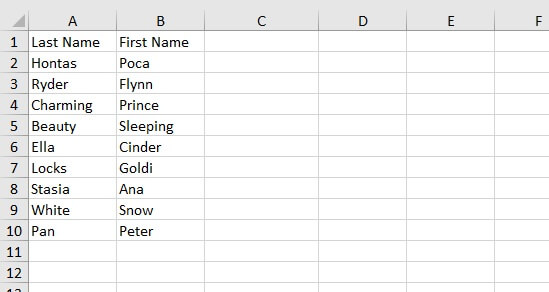
• Highlight the A2 to B10 range, making sure that A2 is the first cell (the active cell) of your selection. 
• Click the “A to Z” icon.

or

• Click any cell within the range.
• Click the “Sort” icon.
• Look at the data range selected by Excel. If it includes the header row, check the “My data has headers” box. This will remove that row from your selection to be sorted.
• Select the column you want to sort by.
• Click OK.

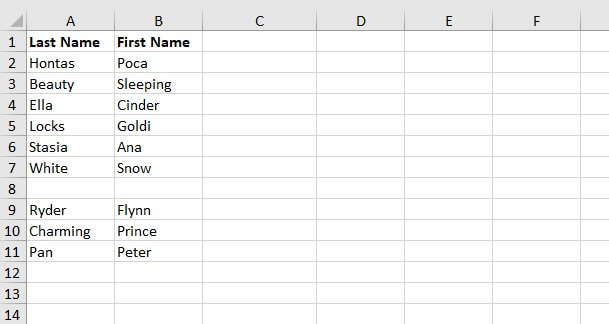
2. Excel only alphabetized a portion of your data set

This likely happened because there was a break, or gap in your data set, which Excel interprets as two separate pieces of data, causing it to ignore anything after the gap.

This is easily resolved by highlighting the entire area to be sorted, and sorting as we’ve learned above.

3. I only want a section of my data set to be sorted

There may be times when you want to do the opposite — sort only one section of an unbroken data set. Let’s use the list below as an example.

Maybe we want to alphabetize by the destination without changing the current order of the names.

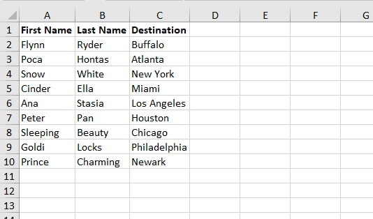
We cannot simply click the “A to Z” icon since Excel will maintain the data across each row. In this case, we must be specific about telling Excel exactly what we want to sort.

• Select the range C2 to C10.

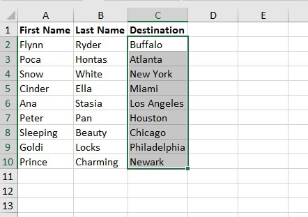
• Click the “A to Z” or the “Sort” icon. A Sort Warning dialog box will appear.

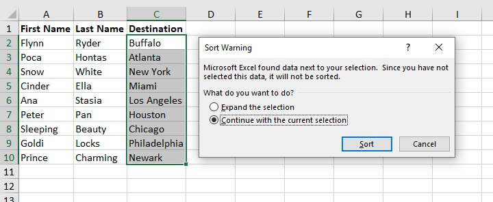
• Since we have deliberately selected only a portion of the data set for sorting, choose the “Continue with the current selection” radio button.
• Click Sort.
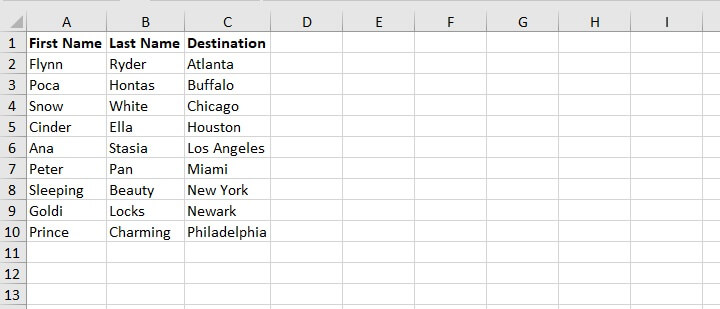
• The original order of our passenger list has not changed, but the destinations are now in alphabetical order.

How to sort alphabetically in Excel with formulas

But what if your data set is a bit trickier, like the one below?

Applying the “Sort” command to this list would simply result in data sorted by the first names since those are the first values in each cell. The only solution in a case like this is to get creative with formulas. This will involve a few steps if we want to maintain the format shown above.

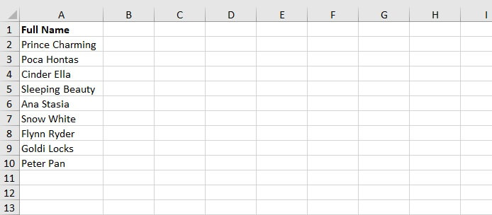
The LEN, LEFT, RIGHT, and SEARCH functions are incredibly useful for manipulating text data, as we’ll see below.

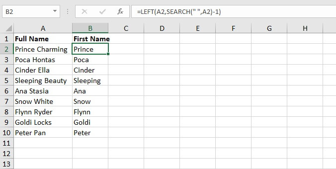
Step 1 - Extract the first names

=LEFT(A2,SEARCH(" ",A2)-1)

This formula searches for and identifies the position of the space character in cell A2. It then subtracts one position from that number and returns the leftmost characters prior to that point.

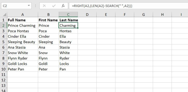
Step 2 - Extract the last names

In the adjacent cell, enter:

=RIGHT(A2,(LEN(A2)-SEARCH(" ",A2)))

This formula uses the LEN function to count the total number of characters in the A2 text string, and identify the position number of the space character. The difference between those two numbers is the number of rightmost characters we want to return as the last name.

Step 3 - Sort as usual

We can now sort by Column C in the usual manner, and

Step 4 - Remove the working columns

Simply delete columns B and C since our original list is now alphabetized.

Summary

There’s no doubt that you will need to alphabetize lists in Excel since it’s one of the more frequently used data organization tasks. Sharpen your sorting skills now with these tips on how to alphabetize in Excel. 

Then move on to more topics in Excel with our Excel - Basic and Advanced course. Or you can start with our free Excel in an Hour course.

Level up your Excel skills

Become a certified Excel ninja with GoSkills bite-sized courses

Start free trial