How to Freeze Panes in Excel

If you’ve worked in Excel, you’ve likely come across spreadsheets that are longer or wider than one screen. If not, that day is coming, trust me. And it may seem like a small thing to some people, but scrolling back to the top or to the left to view the header rows or the first column in your data set gets annoying - fast.

The folks at Excel know how much you hate it when that happens, so they’ve created a command to take care of it: ‘Freeze Panes’. There’s also a similar command called ‘Split’, which works in a different way but is just as useful. They’re both easy to locate, and we’ll tell you exactly how they work.

Before we get started, it’s important to remember that freezing or splitting a worksheet is simply another way of viewing the data that’s on the sheet - it doesn’t change the data that was entered, or how the information will appear when it is printed.

Let’s take a look at a few examples to see how useful these features are. To make this explanation easier to understand, download the practice worksheet and follow along.

What does the Freeze Pane command do?

‘Freezing’ cells keeps them visibly fixed on the spreadsheet even if you’ve scrolled beyond the usual range of that column or row.

Freeze Panes is located on the View tab in the Window command group, which makes sense, since it affects how we view our spreadsheet window.

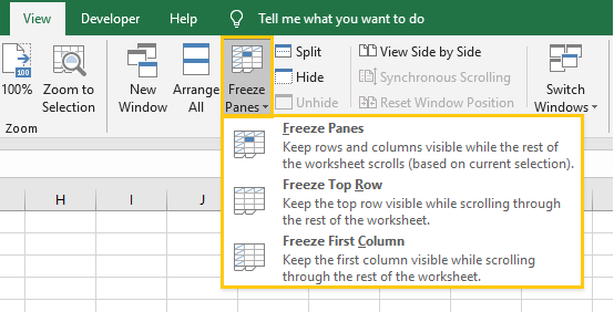
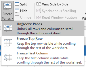
The Freeze Panes command dropdown offers three options:

Freeze Panes - uses the location of the active cell to determine which cells to freeze

Freeze Top Row - freezes the first visible row of the active spreadsheet

Freeze First Column - freezes the first visible column of the active spreadsheet

If you’re using a Mac, these three commands may be shown side-by-side.

Freeze Panes (option 1)

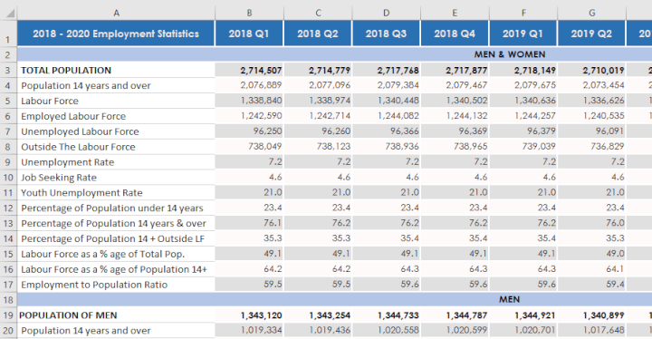
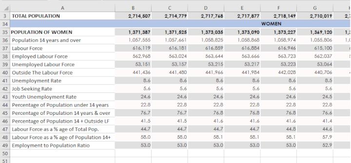
This is a data-rich sheet with several rows and columns. Scrolling to the right or to the bottom will usually result in a situation where we want to remember what statistic is being reported on in that row, or what year and quarter is being referred to in that column.

‘Freeze Panes’ is used when you want to be able to see the visible cells to the top and left of your selection no matter where your scrolling takes you.

Deciding what to freeze is dependent on what we want to keep visible at the moment. Maybe we want to be able to see Rows 1-3 and column A at all times so that we have these reference points when we’re looking at data for subsections of the population. In that case, we select cell B4 as our active cell and click Freeze Panes. 

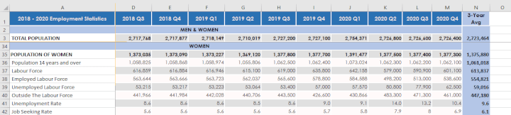
This will ensure that no matter how far down we scroll, we will still be able to see Rows 1, 2 and 3. 

Notice that Excel displays a thin gray line below Row 3 and to the right of Column A to show where rows or columns have been frozen.

Since column A was to the left of our selected cell when the freeze took place, we are always able to see column A, no matter how far right we scroll. This is useful, because our data set extends far right and without scrolling, we would find ourselves unsure of exactly what data is being reported in cell N41, for example.

Freeze Top Row (option 2)

So we’ve figured out what to do if we wanted to freeze multiple rows (in the above case, rows 1, 2 and 3). But quite often, freezing the top row is all you need. If you just want to be able to view your column headings so that you don’t get “lost” while viewing data, click the second option under the Freeze Pane dropdown - Freeze Top Row. 

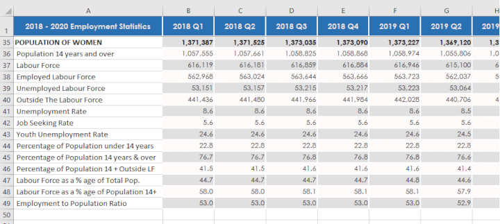
And that’s all there is to it! Now you can scroll down all you want, and Row 1 will remain visible. 

The Freeze Top Row command also applies if you wanted to freeze a single row which isn’t Row 1. For instance, say you wanted to always show Row 3 without seeing rows 1 and 2. Here’s how to do it. 

Scroll your worksheet so that Row 3 is the first row visible, then click the ‘Freeze Top Row’ icon. Boom! You’re done.

You can see from this that Excel interprets “top row” as the first row visible at the time you executed the command. So if you've already scrolled past Row 1, and Row 12 is now the first visible row, guess what? Clicking ‘Freeze Top Row’ will keep Row 12 visible until you unfreeze it again.

Note:

• With the Freeze Top Row command, the first column isn’t frozen, so scrolling to the right will not keep the first column visible.

Freeze First Column (option 3)

The ‘Freeze First Column’ command works in much the same way as ‘Freeze Top Row’. When you select this command, Excel will freeze the first column visible at the time that the Freeze First Column command is executed, regardless of where your mouse is positioned on the worksheet.

By doing this, we’re able to scroll all the way to the right to see the last column of data and still view Column A. 

Notes: 

• Excel interprets “first column” as the first column visible at the time you executed the command. So if you've already scrolled past Column A, and Column E is now the first visible column, then clicking ‘Freeze First Column’ will keep Row E visible until you unfreeze it again.
• With this method, the first row is not frozen, so scrolling downward will not keep the top row visible.

Unfreeze rows or columns

If you realize that you’ve frozen rows or columns on your worksheet at the wrong spot, or if you’re done working with your data and you’re ready to restore your sheet to its normal view, unfreezing panes is just a click away. 

Simply go back to the View tab, click the Freeze Panes dropdown and click ‘Unfreeze Panes’. (It will be the first option if you have any rows or columns frozen.)

What does the Split command do?

Similar to freezing, when you ‘split’ a worksheet view, you have a similar desire to keep a certain portion of the spreadsheet visible, regardless of how far away you’ve scrolled from that point. However, a key difference between freezing panes and splitting them is that splitting gives you the flexibility to scroll on either side of where the sheet has been split, so that you are still potentially able to view the entire worksheet.

Remember that when you’ve frozen panes, cells above and to the left of the frozen area are not scrollable, and may even be hidden.

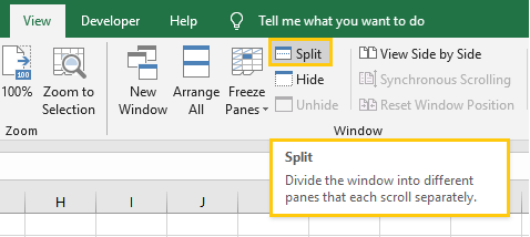
The ‘Split’ command is right next to ‘Freeze Panes’ on the View tab of the ribbon.

Let’s see how we can apply a split view to a customer database worksheet.

Horizontal split

Let’s say you want to be able to apply a horizontal split to compare data by rows. Just position your mouse in any column A cell except A1 (you’ll see why later) and click the Split icon. This creates a horizontal pane on your worksheet and two sets of scrollbars (look to the right of your spreadsheet). The horizontal pane allows you to view different sections of your worksheet simultaneously, and, unlike ‘Freeze Panes’, allows you to click on any pane to make it the active one, and scroll using the scrollbar or mouse wheel as usual.

Vertical split

If you want to apply a vertical split to compare data by columns, position your mouse in any row 1 cell except A1 (again, you’ll see why later) and click the Split icon. This creates a vertical pane on your worksheet and two sets of scrollbars (look to the bottom of your spreadsheet). The vertical pane allows you to view different sections of your worksheet simultaneously, and, unlike ‘Freeze Panes’, allows you to click on any pane to make it the active one, and scroll using the scrollbar or the left and right keyboard arrows as usual.

Four-way split

You can even split your worksheet into four copies by going to cell A1 and clicking Split from the View tab. 

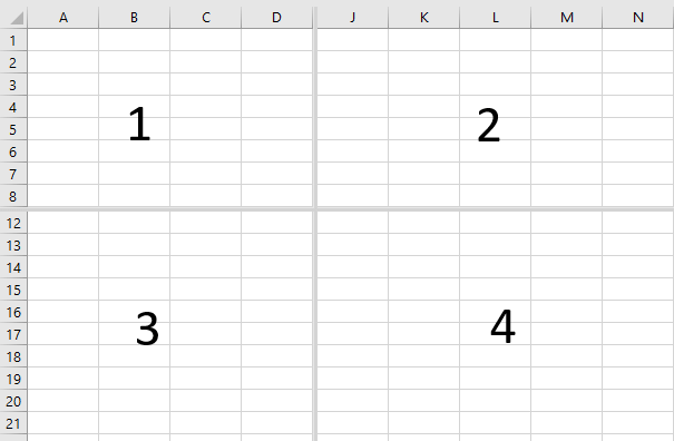
How is this useful, you ask? Remember how you could only scroll up and down with the horizontal split, and left and right with the vertical split? Well, splitting your screen into four parts gives you the flexibility of scrolling up or down, left or right regardless of which quadrant you’ve selected.

Let’s say you click on a cell in Quadrant 1 as illustrated above. Scrolling from top to bottom will scroll both Quadrants 1 and 2 up and down. If you scrolled from left to right while a cell in Quadrant 1 is selected, this would scroll Quadrants 1 and 3 from side to side.

Note: If you click the ‘Split’ command while A1 is the active cell, Excel will split your screen into four equal parts. But you can either:

1. position your mouse where you’d like the split to take place, then click the ‘Split’ command, or
2. drag and drop the split bar to anywhere you’d like after Excel does the split.

Remove a split screen 

You can cancel or remove a split screen in Excel by de-selecting the Split icon, or simply by double clicking the split bar(s).

Troubleshooting - Split or Freeze Panes

If you find that even after this wealth of knowledge about how to freeze panes and split your worksheet view in Excel, you’re still having problems, here are some troubleshooting tips to note:

1. If your ‘Freeze Panes’ icon is grayed out, most likely your worksheet is in Page Layout view. From the View tab, go to the Workbook Views command group and click either Normal or Page Break Preview, and the ‘Freeze Panes’ command will be enabled.
2. You cannot split and freeze a worksheet at the same time. 
3. The ‘Freeze Panes’ command is not available in Excel Online.
4. If you clicked ‘Freeze Top Row’ or ‘Freeze First Column’ and now you can’t see Row 1 or Column A, it likely wasn’t visible at the time you executed the command. Click the ‘Unfreeze’ command, and make the row or column you want to see visible at the time you re-execute the command.

Summary

And there you have it - no more scrolling up, down or across to see what that row or column was all about. Want to learn more useful tips to Excel in your life? Check out our course library or browse our other resources to learn more.

Level up your Excel skills

Become a certified Excel ninja with GoSkills bite-sized courses

Start free trial