
There’s nothing like mastering a good hack—particularly learning a Microsoft Excel hack.
Learning to manipulate and analyze tons of rows of data is enough to make anyone go cross-eyed. So, who wouldn't want a trick that promises to save you time, stress, and elbow grease?
Well, today’s your lucky day! We’ve rounded up 11 different Excel hacks you’re sure to use and love. It won’t be long before you’ll wonder how you ever survived without them.
Ready to become a certified Excel ninja?
Start learning for free with GoSkills courses
Explore Excel courses1. Familiarize yourself with keyboard shortcuts
Alright, perhaps this first one doesn’t count as just one hack. However, if you’re looking for a surefire way to save yourself time and frustration in Excel, it pays to familiarize yourself with some different keyboard shortcuts.
There are hundreds (yes, literally hundreds) that you can use. So, the best thing to do is to take note of some of the common tasks or actions you’re taking in Excel, and then seeing if there are existing keyboard shortcuts for those.
Want a handy resource? We already pulled together a list of 200 Excel shortcuts for PC and Mac that you can reference!
Download your free shortcuts PDF cheat sheet below.
Learn the best Excel shortcuts!
Download our printable shortcut cheatsheet for PC and Mac.
Here are a few of our favorites:
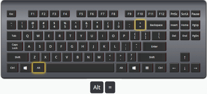
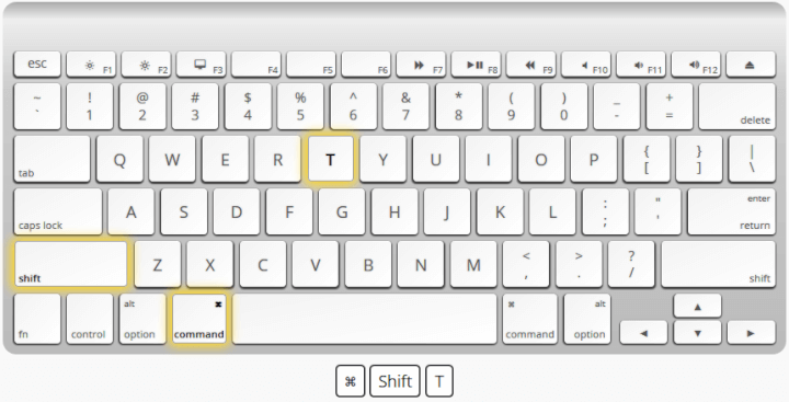
Autosum all selected cells
Speed up your number crunching by quickly summing numbers in a contiguous range.
PC: Alt =
Mac: Command Shift T
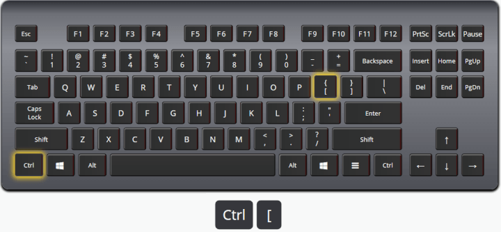
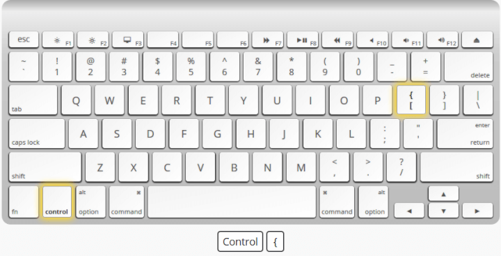
Select direct precedents
Select a cell with an active formula and see which cells are directly referenced by that formula.
PC: Ctrl [
Mac: Control {
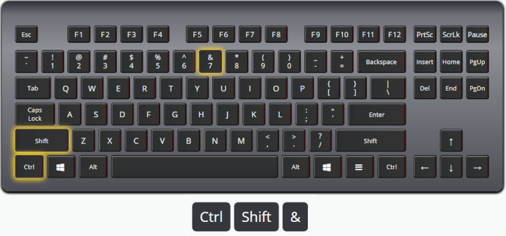
Add a cell border
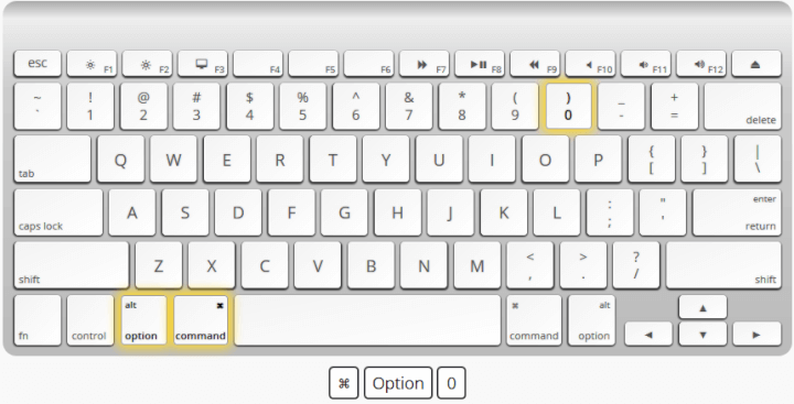
Save yourself some clicks when formatting by instantly adding a cell border. This works with one or multiple cells selected.
PC: Ctrl Shift &
Mac: Command Option 0
2. Select all cells with one click
Have hundreds (or even thousands) of rows of data—and need to select them all?
You can give yourself a finger cramp from tons of endless clicking and scrolling. Or, you can use this simple trick to select all cells with one single click.
All it takes is clicking on that light gray triangle that appears in the top left corner of your spreadsheet. Click it once, and every single cell in the spreadsheet will be selected. It’s as easy as that!
3. Instantly resize columns and rows
There’s nothing worse than having your text run outside of the width of the column. And, needing to click and drag to resize the column to the perfect width over and over again can be a pain.
Fortunately, you can do this instantly. Place your mouse on the line between two column markers (C and D, for example) until you see a symbol that looks like two opposite-facing arrows.
With that symbol, double click on that line that separates the columns, and the column will automatically be resized to fit the widest piece of text within that column.
Note: The same hack can be used to adjust the height of rows!
4. Easily format numbers
Let’s say that you have an entire column that contains digits that represent the same thing—like dollar amounts, for example.
Right now, there isn’t a dollar sign displayed in front of each number, and you’d like to insert one there. There’s no need to do this one at a time.
Simply select the column that contains the digits you want to re-format, and then use the below keyboard shortcut to automatically format that entire column to dollars:
Ctrl - Shift - $
With that simple trick, your entire column will be displayed with the dollar sign, any necessary commas, and two points after the decimal point.
Note: The same trick works for percentages! Just hit Ctrl - Shift - % to include the percent sign with each digit.
5. Move up without scrolling
When you have a particularly large data set, you know that it takes a while (and quite a bit of scrolling) to get all the way to the bottom of your worksheet. And, when you’ve finally made it? The last thing you want to do is scroll all the way back up to the top.
Pushing Command (Ctrl on a PC) and the up arrow twice will bring you back to the top of your spreadsheet.
Why do you have to hit the up arrow twice? Hitting it once will bring you to the last row of data that appears before an empty row (which, in this case, is the last line of our data). Hitting the up arrow twice brings us all the way back to the top.
So, to summarize:
Command (or Ctrl on a PC) + Up Arrow Once: Brings you to the last line of data that appears before a blank row
Command (or Ctrl on a PC) + Up Arrow Twice: Brings you to the top of your worksheet
Note that this shortcut works on Excel for Mac and PC 2016. Shortcuts on Mac may vary depending on your OS, or on older versions of Excel.
6. Apply the same formatting
Let’s say that I need to create another column in my spreadsheet—and I want to apply the same formatting that’s in an existing column. For example, I want the “Total” column I’ve created to also have bold font and the dollar signs like the “Price Per Gallon” column that already exists on my spreadsheet.
It’s simple to apply existing formatting to a new column.
Select a cell that has the formatting you want and copy that cell. Then, select the section of your spreadsheet that you need to apply that formatting to, right click, select “Paste Special,” and then click the box for formats.
Now, when I enter a value in that “Total” column, it’ll automatically appear with bold font and a dollar sign—without me having to do any further manual work.
7. Insert more than one row or column
Needing to insert one row or column at a time can be monotonous. Luckily, there’s a quick trick that allows you to insert multiple rows or columns into your spreadsheet with a single click.
This hack is painfully simple: Highlight the number of rows or columns that you want to insert, and then right click and select insert.
So, if I want three new, blank columns to appear ahead of my existing “Gallons Sold” column, I would highlight three columns starting with “Gallons Sold” and then click insert.
Just like that, I have three brand new columns in my spreadsheet—without the hassle of inserting one at a time.
Note: This trick works the very same way with rows. You’d obviously just highlight rows instead of columns.
8. Make a copy of your worksheet
If there’s a worksheet that you find yourself creating regularly—like a monthly report, for example—needing to re-create it from scratch every single time isn’t necessary.
Instead, it’s better to make a copy of your entire worksheet, so that all of your formatting and other elements are already there—you just need to swap out any necessary information.
To do this, right click on the tab for your worksheet at the bottom and select “Move or Copy.” At that point, you’ll be met with a popup that asks where you’d like your sheet to be moved and where you’d like it to appear.
In this example, I want my copied sheet to live in my same workbook, and before my existing “Beer Sales Data” worksheet. So, I select those options, check the box for “Make a Copy,” and end up with an exact replica of my existing sheet to use and revise:
9. Embed an Excel spreadsheet
If you’re putting together a proposal, report, or other important document in Word, it can be helpful to embed the contents of your Excel spreadsheet.
This is fairly easy to accomplish. To do so, select and then copy the portion of your spreadsheet that you want to embed.
Head to Word, and then select “Paste” and “Paste Special.” Within that popup, find and select the option for “Microsoft Excel Worksheet Object,” ensure you select the option for “Paste Link,” and then click “OK.”
You will see your spreadsheet embedded in your document (you’ll likely need to do some brief resizing!). Additionally, since you selected the “Paste Link” option, whenever you make changes to your spreadsheet, they’ll automatically be updated in the embedded chart in your Word document. Pretty slick, right?
Note: You can also embed an excel spreadsheet in an email. But, the exact directions for that will vary depending on your email provider.
10. Find and replace values
Maybe you noticed an error in your spreadsheet. Or, perhaps you want to update some terminology.
There’s no need to scroll through your entire data set to find each individual occurrence of that term or value. Using the “Find and Replace” feature can help you update everything at once.
Highlight the cells you want to search and hit Ctrl + F. You’ll be met with a popup where you can enter which term you want to find in the spreadsheet, as well as what you’d like to replace it with.
For example, if I wanted to replace the appearance of “Stout” with “Vanilla Stout,” I could use “Find and Replace” to do that in a few short steps.
 Note: It’s important to be aware that this feature will replace every appearance of the combination of letters that you enter. So, if you had a list of states and wanted to replace CO with AZ, it would replace anywhere that “Co” appears—meaning you could end up with something that says “Azmpany” instead of “Company.”
11. Use two windows
Do you have worksheets within the same workbook, but would like to view them side by side—rather than needing to click back and forth between the two?
Of course, there’s a way you can easily do this.
If you’re on a Mac, click “Window” within the main Excel menu and then select “New Window.” If you’re on PC, go to “View” in the Excel ribbon and then select “New Window.”
Doing so will open your existing workbook in an entirely new window—so you can position them side by side and avoid a bunch of clicking.
The best part? Any changes you make will be applied to both windows—so you don’t need to make changes twice.
Want even more hacks?
These simple tips will undoubtedly help you save some time in Excel. But, we haven’t even touched on some of Excel’s more advanced features—like pivot tables and macros—that can help you take a lot more elbow grease out of using spreadsheets.
Has learning Excel improved your efficiency at work? We'd love to hear from you! Send us an email or reply in the comments below.
Eager to know even more? Sign up for our Excel course, roll up your sleeves, and prepare to impress everybody with your Excel mastery.
Ready to become a certified Excel ninja?
Start learning for free with GoSkills courses
Explore Excel courses