Excel Challenge 38: Data Lookup From Multiple Sources

Ready for Excel challenge #38?

Everything you need to participate in the challenge can be found on this page. To take part:

1. First, watch the challenge video and read the instructions below the video.
2. Review the previously published video(s) and article(s) on which the challenge is based.
3. Download the Excel worksheet you will use to complete the challenge tasks.
4. Put yourself to the test!

Want to chat about your approach and process with other Excel heads? Join our Slack channel to share your insights and questions with like-minded learners.

---

The challenge🤺

Here’s the scenario to be solved from the download file:

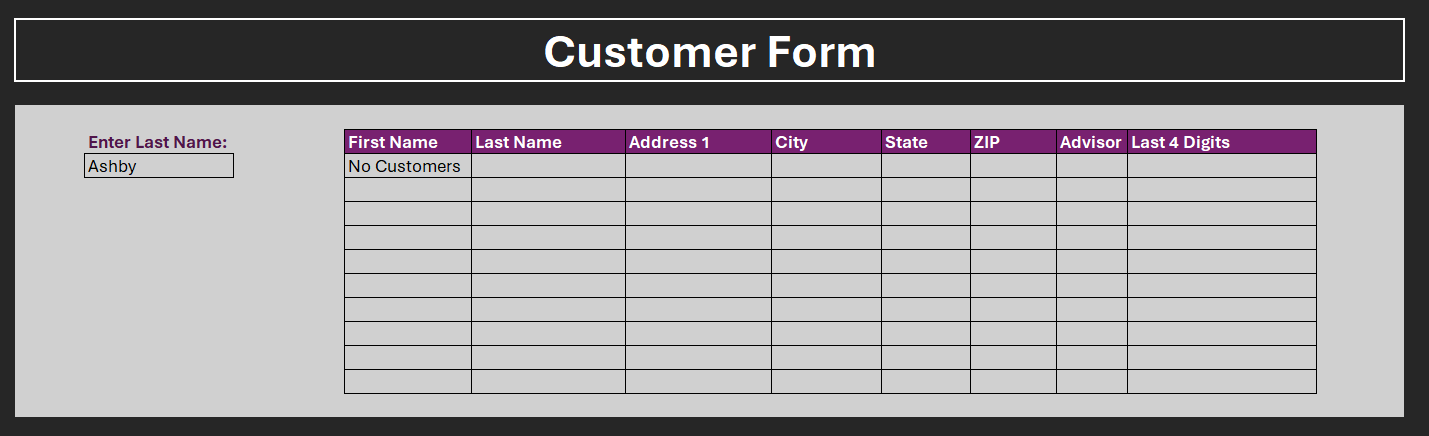
At an inbound contact center, the agents' job is to take customer calls and direct them to the correct sales advisor. 

They want to be able to type the customer's last name into a form and the form returns all customers that match. They can then use the last 4 digits of the credit card number on file and the customer's first name to confirm their identity and direct them to the correct advisor. 

The data will be coming from our consolidated customer list on the worksheet ‘All Customers’. 

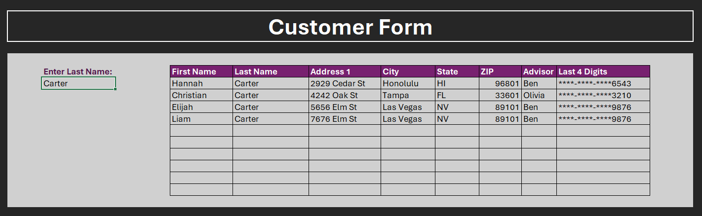
You are the Excel expert in the office! Can you set this up?

Things to note:

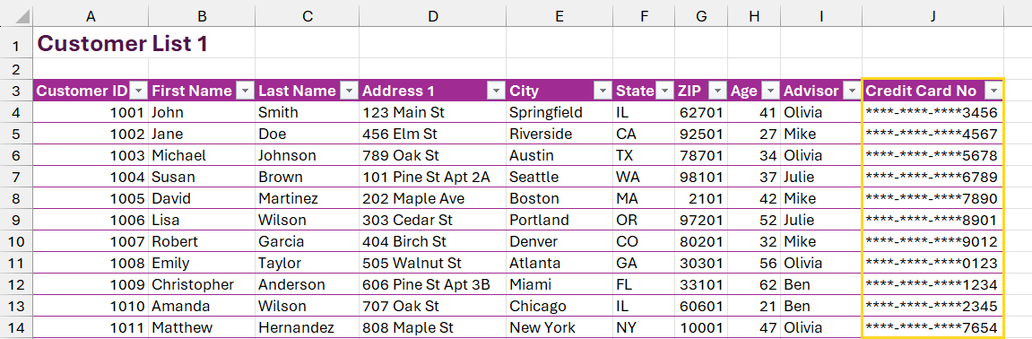
1. Our customers are split across two worksheets, ‘Customers 1’ and ‘Customers 2’. 
2. In the workbook, the full credit card number is shown. 
3. The form excludes the columns ‘Customer ID’ and ‘Age’. 

---

Tasks🏋️

1. Format the datasets as Excel tables.

First, we need to format the datasets on ‘Customers 1’ and ‘Customers 2’ as Excel tables. 

• Name the tables ‘Customers1’ and ‘Customers2’ respectively. 

2. Mask the credit card number.

Next, we need to use a formula to mask all digits in the credit card number EXCEPT the last 4. The masked digits should be replaced with asterisks, e.g. ****-****-****-1234.

• Think about what text formula allows you to extract characters in Excel. 

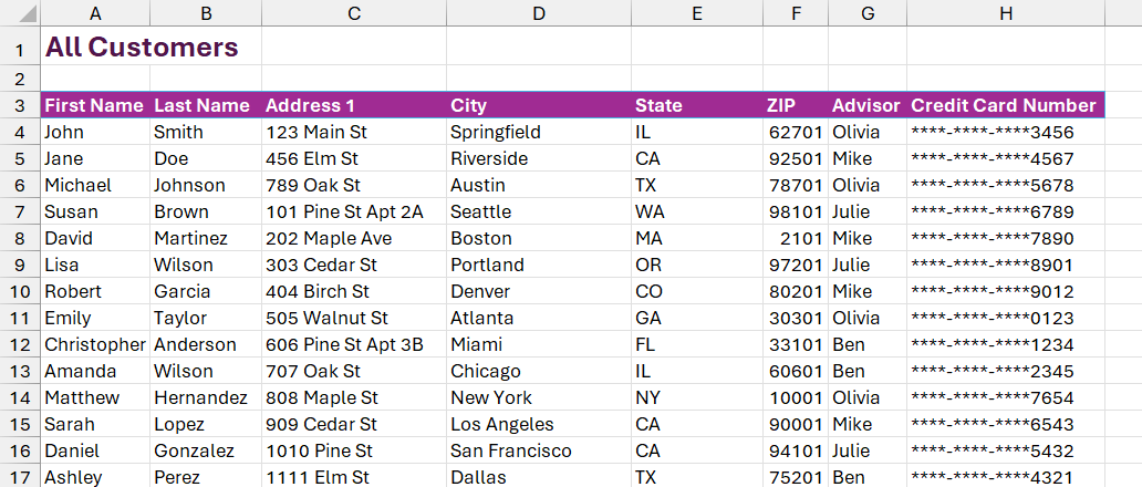
3. Combine the datasets

We need to combine the data in the ‘Customers1’ table and the data in the ‘Customers2’ table into one consolidated customer list on the ‘All Customers’ worksheet. 

NOTE: To combine the datasets, you can use formulas, Power Query, or you can manually copy and paste the data. Please try to use Power Query or formulas to practice those skills. In this example, I will be using formulas. 

• Think about what dynamic array formula we could use to vertically stack arrays. 

4. Remove columns

Next, we need to remove any columns that are not needed in the form. Notice that the columns ‘Customer ID’ and ‘Age’ are not returned on the form. 

NOTE: To remove the columns, you can use formulas, Power Query, or you can manually delete the columns. Please try to use Power Query or formulas to practice those skills. In this example, I will be using formulas. 

• Think about which dynamic array formula we could use to choose only the columns we want to keep. 
• Columns are numbered left to right, e.g. 1, 2, 3 etc.  
• Once complete, we need to update the column headings to match the new data. We can do this manually. 

5. Add the formula to the form

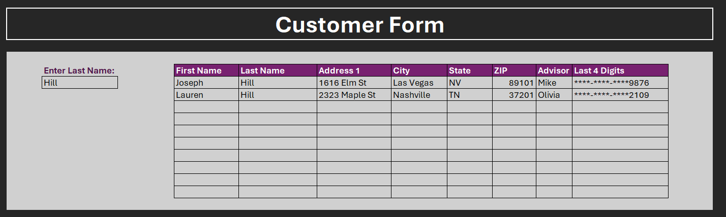
Finally, we need to add a formula to the form that will return results from dataset on the ‘All Customers’ worksheet depending on what name has been typed into cell C6. 

• The formula should be a dynamic array formula that has spill capabilities to account for multiple customers with the same last name. 
• Ensure that the formula includes contingency if the wrong name is entered, there is a spelling mistake, or the customer doesn’t exist. 
• Test to make sure the formula is working by typing different names from the dataset into cell C6. 

If no customer is returned, the result should look like this. 

So, what do you think? Easy-peasy? Or too tough to tackle? Tell us how you would solve this, then tune in next week for my solution.

We hope you'll enjoy working on this challenge!

---

The solution🎉

---

We hope you enjoyed taking part in this challenge!

Stay tuned to the GoSkills Excel Resource hub for more Excel challenges, and check out our range of expert-led Excel courses for all skill levels to further sharpen your skills.

If you enjoyed this challenge, you’ll love our Basic and Advanced Excel course, which will help you learn both essential and new Excel functions, as well as help you learn practical, real-world skills!

Level up your Excel skills

Become a certified Excel ninja with GoSkills bite-sized courses

Start free trial