Power Query Tips: 10 Most Useful Commands

In the modern business world, every job is now part data analyst. Whether you're in HR, sales or marketing you need data skills. Anyone who has worked with data knows, that it rarely comes in the format they need. It usually requires some extra work to get it into a workable state.

Power Query in Excel is the solution to all your messy data problems. It can do so many useful data transformations that will help clean your data so that it's ready to be used for further analysis.

In this post, we'll go through some extremely useful Power Query tips to help you use the best data transformation features available in the software.

If you've never heard of Power Query and want to get familiar with what it can do, then check out this quick intro video:

For a more in-depth look at the software try taking the GoSkills Power Query course or check out this introduction to Power Query article.

Okay, let's dive right in!

1. Split cells by delimiter

Here's the scenario:

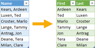
The data contains a list of names and they're all formatted the same way. Last name followed by a comma and space and then the first name.

But you need the first and last name separated in their own columns. You can do this with Power Query's split column command.

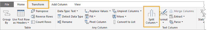In the query editor, select the column you want to split and go to the Transform tab. Select the Split Column command from the ribbon and choose by Delimiter.

You can also access this by right-clicking on the column heading and selecting Split Column from the menu.

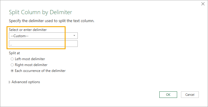Choose a Custom delimiter and enter a comma followed by a space character. Now press the OK button. Now the names are all separated into their own columns. Easy!

2. Fix country-specific  formatting

Ok, here's the deal:

Different countries use different formatting conventions for things like dates and numbers.

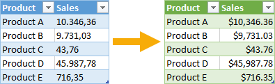
In Germany and many other mainland European countries, $10,346.36 would be written as $10.346,36. In this number formatting, the comma and period play the opposite role and Excel will treat this as text instead of a number.

Dates can be another tricky situation. In the US they use a mm/dd/yyyy format while the rest of the world uses the dd/mm/yyyy or yyyy-mm-dd format.

This can be extremely frustrating when trying to work with data received from different locations across the world.

Power Query's locale functionality can make this a breeze to fix.

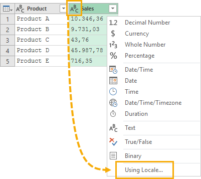Left-click on the data type icon found in the left-hand side of the column heading. Choose Using Locale from the menu.

You can also access this by right-clicking on the column heading and selecting Change Type from the menu.

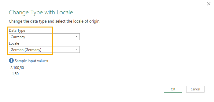Select the Data Type that you're trying to transform. In this case, it's a currency.

Now, select the Locale where the data came from. In this case, it's been formatted using the German locale. Press the OK button and Excel will now recognize the data as numbers instead of text!

3. Fill in missing data

This is one of the Power Query tips on this list you might find yourself using almost daily.

You might have missing data in some rows and need to fill down the data from the row above.

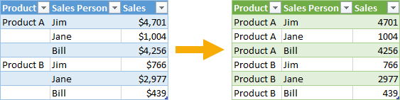
This happens a lot when people copy and paste data from a pivot table.

In this case, the outer leftmost column has only the first row populated and blank rows beneath representing the same product. Luckily filling this data down the column is easy with Power Query.

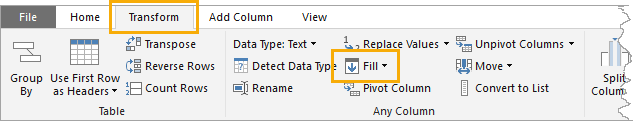Select the column which you want to fill down data in and go to the Transform tab in the Power Query editor ribbon, then press the Fill command and choose Down from the menu.

This can also be used by right-clicking on the column and selecting Fill and Down from the menu.

This will fill any blank cells with the last non-blank cell found above. Voila, no more missing data!

4. Reorganize your data by moving or removing columns

Your data might be exactly the way you want it with one minor detail missing. Its got columns you don't really need or the order of the columns isn't how you want to view them.

It's a simple thing, but de-cluttering and organizing your data means you can focus on the important stuff.

This can easily be fixed when importing data with Power Query.

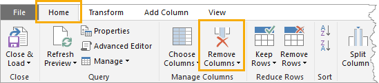Select any column you want to remove from the data and go to the Home tab in the query editor ribbon and select the Remove Columns command, then choose Remove Columns from the menu.

This can also be done by right-clicking on the column and selecting Remove.

Tip: Do the column headings which you want to remove sometimes change? Then select the columns you want to keep and use the Remove Other Columns command instead. The query will reference the columns you want to keep and won't cause errors if the columns you remove change names the next time you import data.

Moving columns is easy too! Just left-click on the column heading and drag it to the new location either left or right.

5. Remove duplicate data

Removing duplicate data is an essential trick you need in your data arsenal.

Duplicate data can be very dangerous. Accidentally doubling up the reported sales in your company could have catastrophic results.

It may not be as serious as needing to get rid of duplicated data. You may just need to extract a list of unique values from a column with repeats.

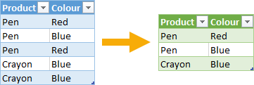
Whatever the reason for needing to remove duplicates, Power Query makes it dead easy.

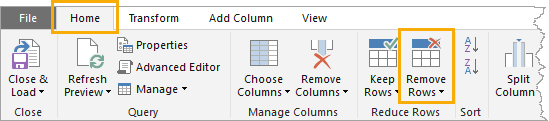Select the column or columns which contain the duplicate data, then go to the Home tab in the Power Query editor ribbon and press the Remove Rows button. Select Remove Duplicate from the menu.

You can also access this by right-clicking on the column heading and selecting Remove Duplicates from the menu.

No more duplicates!

If you want to keep a record of the data that was duplicated, there's even a command for that. In the Home tab, use the Keep Rows command and select Keep Duplicates from the menu.

6. Group data

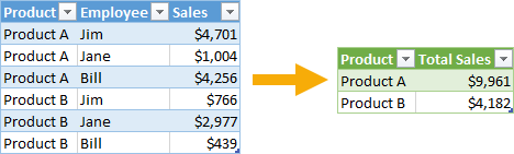Power Query allows you to summarize your data with the Group By command.

Summarizing data is the key to gaining insights, but if you're looking to analyze your data it's better to avoid this command and do any summarizing inside a pivot table later. Using a pivot table is a much more dynamic approach.

Grouping can still be a useful or needed step in your data transformation process.

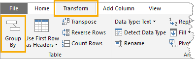To group your data, go to the Transform tab in the Power Query editor ribbon and press the Group By command.

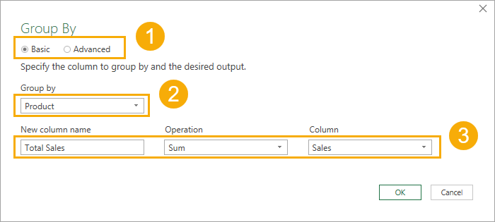Configure the group by options.

1. Choose either the Basic or Advanced options. The basic options will allow you to group your data by a single field whereas the advanced options will allow for more than one field.
2. Select the fields you want to group by. This will usually be a text or date-based field.
3. Select the columns you want to summarize and the operation which you want to summarize them by. These will usually be numerical fields which you want to sum, count or take the average from.

7. Transpose your data

Your data is looking good, but...

You just want to flip it around.

What you need to do is transpose it. This means the rows become columns and the columns become rows.

Transposing the data is going to be a 3 step process. Part of the data that needs to be transposed is in the column headings so you'll need to turn these into a row of data first.

1. Go to the Transform tab and press the Use First Row as Headers command, then choose Use Headers as First Row from the menu. This will get the column headings into the first row of data.
2. In the Transform tab press the Transpose command.
3. Now you can promote the top row back to column headings. In the Transform tab, press the Use First Row as Headers command then choose Use First Row as Headers from the menu.

8. Calculate age

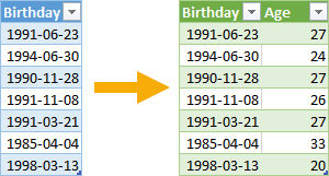Calculating someone or something's age is a common need in any type of analysis, and Power Query has this calculation built in.

Select the column containing the date which you want to calculate an age based on.

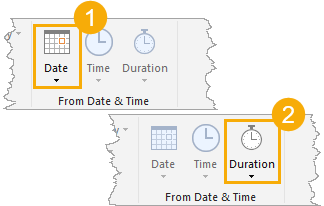
1. Go to the Add Column tab in the Power Query editor and press the Date command and choose Age from the menu. This will give the age in days so you'll need to convert this to years.
2. Go to the Transform tab in the Power Query editor and press the Duration button and choose Total Years from the menu.

Now you've got the age in years! When you refresh the query, the calculation will update based on today's date.

9. Unpivot data

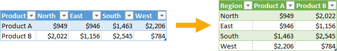
Your data might come already pivoted.

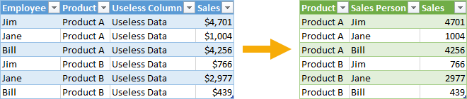
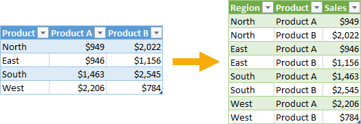
All the values in the Product A and Product B columns represent the same metric of sales. They should really be in one column with another column that tells us what product the sales amount was from.

In its current format, you won't be able to further analyze the data. In this case, you need to un-pivot the data.

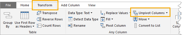Select any columns which you want to un-pivot then go to the Transform tab in the Power Query editor ribbon and select Unpivot Columns from the Power Query editor ribbon.

Now a new column with either Product A or B will appear along with all the sales figures in another column.

You'll need to rename these columns as by default they will be called Attribute and Value. Rename them to something like Product and Sales respectively.

Your data is ready to be loaded into a pivot table for further analysis now!

10. Create a  column based on examples

One common scenario is creating new columns based on existing columns in your data.

In this example, you have a list of email addresses and you want a new column that contains text saying "Ardeen works at Uber" and so on, for each row.

You need to extract the first name and the company from the email address and concatenate them together while capitalizing the name and company.

This would require applying a few different transformation steps in Power Query to obtain the result.

This means you have to figure out which series of steps will get the result you want.

You can actually get Power Query to figure out how to transform the data based on a couple of examples you provide.

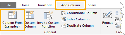Go to the Add Column tab of the Power Query editor ribbon and select the Column From Example command.

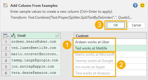Now you need to give Power Query a few examples of the result you want in the column.

1. Give 2 or more example row results for Power Query to learn and create the desired transformation.
2. Power Query's guess at the transformation will appear in light gray down the remaining rows. Check the results and add more examples if it's not quite correct.
3. Press the OK button when you're satisfied with the results.

Power Query creates and adds the needed transformation steps to your query!

You have the power

Power Query has a lot of data transformation commands built in.

If you need to transform your data in some way, Power Query probably has a command for it!

If you're looking for more Power Query tips then check out this list.

Getting clean data formatted exactly how you want is now easy. No complex coding or formulas required.

Ready to unlock the "power" in Power Query? Take the GoSkills Power Query course and get a resume-boosting certificate when you are finished.

Start working with data like a pro

Take the Power Query course today!

Take the course