Excel Challenge 58: Customer Segmentation Using One Formula!

Can you build a clean customer segmentation report with a single formula that spills a three-column result?  Everything you need to participate in this Excel challenge can be found below. To take part:

1. Watch the challenge video and read the instructions below the video.
2. Review the previously published video(s) and article(s) on which the challenge is based.
3. Download the Excel worksheet you will use to complete the challenge tasks.
4. Put yourself to the test!

The scenario 🖼️

Elif is a Marketing Analyst at a busy retail company. Her manager needs a quick segmentation view to design loyalty programs and promotional campaigns.

---

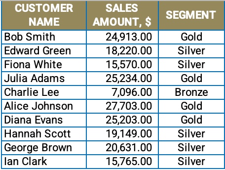
Show how much each customer spent last quarter and classify them as Gold, Silver, or Bronze so we can reward them according to spend.

---

Your mission: create that summary in a single formula — no helper columns, no manual steps.

The data set 📊

Each transaction row contains:

• Customer Name

• Product

• Quantity

• Sales Amount, $

• Date

The task 🏋️

In one spilled formula, produce a three-column report:

1. Customer Name (no duplicates)

2. Total Spend across all their transactions

3. Segment label using these rules:

   • Gold → above $22,000

   • Silver → between $12,000 and $22,000 (inclusive of $12,000 and $22,000)

   • Bronze → below $12,000

Your final output should be a dynamic range that expands and contracts with the data.

The rules 📌

• ✅ One formula only (it should spill the full 3-column result)

• ✅ No helper columns

• ✅ Works if new transactions are added to the table

The clues 🕵️

Here are some nudges in case you're stuck:

• Think dynamic arrays, like: UNIQUE, SORT, HSTACK, TAKE, or CHOOSECOLS.

• Aggregate spend per customer with a vectorized approach, such as SUMIFS against a spilled list, or wrap with BYROW if needed.

• A user-defined function (e.g. LET, LAMBDA) might help in keeping your formula readable.

• Remember: your single formula should return three columns. If you’re newer to dynamic arrays, start by getting the customer list to spill — then layer in the total, and finally the segment. Learn more about nesting Excel formulas.

Put yourself to the test! ⏱️

• Build your one-formula solution

• Share your formula and a screenshot of your result!

Advanced challenge 🏋🏼

If you'd like to step up your game, think about how you would:

• 💪 sort customers by Total Spend (descending) in the same formula

• 💪 adapt the same one-cell pattern for top-N customers, or additional tiers.

Expert's solution 🤓

Here is my take on this challenge.

Join the conversation 💬

Want to compare approaches or brag about your solution? Post your formula, why you chose it, and any tricks you used in the GoSkills community on Slack.

GoSkills' most popular course — Microsoft Excel Basic & Advanced with MVP Ken Puls — has an entire section dedicated to understanding dynamic arrays. Start building your skills now!