Working With Excel Dynamic Arrays

---

The Excel community has been pretty excited about dynamic arrays since Microsoft made a general release in January 2020. 

Excel dynamic arrays have changed the way we use all functions and formulas in Excel for the better. For simplicity, we’ll use “Dynamic Excel” to refer to the new environment and “Pre-Dynamic Excel” to talk about Excel’s prior behavior.

What is “dynamic array” in Excel? 

To understand dynamic arrays, we need to understand how formulas work in Pre-Dynamic Excel. Generally speaking, one formula returns an output to one cell. When formulas referred to a range, they were still programmed to return a single value per entry. Even the seeming exception - CSE, or array, formulas (see below) - required knowledge of the expected size of the output range.

In Dynamic Excel, Excel will automatically output a multi-value, dynamic range if that is the result of your formula. A good example that illustrates the difference between Pre-Dynamic and Dynamic Excel is the FREQUENCY function. 

---

---

Control+Shift+Enter (CSE) vs. dynamic array

FREQUENCY is an array function. For any version before Excel 365, that means you’ll have to first highlight the range of cells where the resulting list will be displayed. Then type the formula using the FREQUENCY function syntax. 

It’s important that you do not press Enter. Press CTRL+SHIFT+ENTER. This will let Excel know that you are entering an array formula. Excel inserts curly brackets around the formula. This is to remind you that this was entered as an array formula.

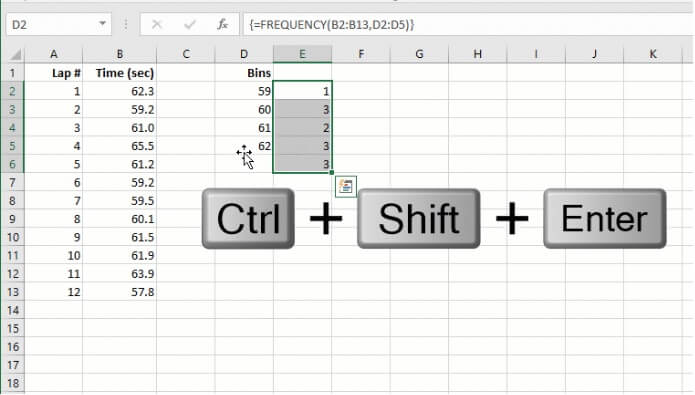If you have a current version of Microsoft 365, Excel recognizes FREQUENCY as an array function. Since Excel 365 operates in a dynamic array environment, you can just enter the formula in the first cell of the range you would like to be your output range. Then press ENTER as normal, and the results will be displayed in multiple cells.

Dynamic Excel makes using array constants easier too. Now when you enter array constants in a formula, Excel understands how to process the operation without any special intervention.

=B3:B6*{1.3,1.6}

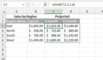The curly brackets around the array constants are manually entered and are interpreted by Excel as a one-dimensional vertical array. This is not new. However, the ability to spill the results without having to enter the formula using Control+Shift+Enter is. Admittedly, entering CSE formulas was always a bit awkward.

From these examples, it can be seen why CSE formulas are on the way to being phased out altogether.

Availability in Excel versions

With all the buzz around Excel dynamic arrays, you’ll probably want to see what all the fuss is about. Here are a couple of things to bear in mind:

1. Dynamic arrays are not available in versions before Excel 365, so, unfortunately, they are not available in Excel 2019.
2. There are eight new functions with which the dynamic array functionality comes built-in.
3. Dynamic array functions and formulas are available in Excel 2021 and Excel Online.

Features

There are three particularly noticeable features of Dynamic Excel: automatic spill behavior, the spill range operator, and the implicit intersection operator.

1. Spill behavior

When dynamic array formulas automatically return values into multiple cells based on whatever output is required, this behavior is called spilling. Spilling has several advantages, including: 

• Excel determines and applies the required output area without any change in the way the formula is entered.
• When source data changes, spilled results will immediately update.
• Reduced need for absolute and relative references.
• Reduced need to copy formulas in a data set. 
• Ability to easily create data validation lists and named ranges that update when lists expand or contract. 

The output area of a dynamic array formula is called the spill range. The spill range is identified by a rectangle around the output area when at least one of the cells is selected. 

Similar to pre-Dynamic Excel CSE formulas, only the first cell in the spill area is editable. Formulas in the other cells appear grayed out and cannot be modified. Any attempt to modify “ghosted” cells within the spill range will destroy the range and will result in a #SPILL! error.

2. Spill range operator

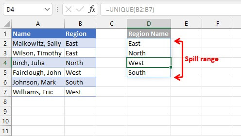
Excel has introduced a spill range operator, #, to denote the output of a spilled array. For example, D2# refers to the spill range beginning with cell D2, which was populated using the dynamic array formula UNIQUE(B2:B7). The formula in cell E2 makes reference to the values in cell D2:D5 with the expression D2#.

=COUNTIF(B2:B7,D2#)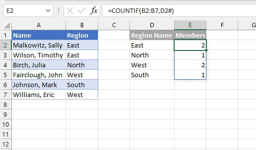

3. Implicit intersection operator

Implicit intersection logic is not new. Excel has been doing this in the background with Pre-Dynamic Excel. In Excel tables, the implicit intersection operator, @, has long been used to indicate an operation that refers to a value in the same row as the formula. Implicit intersection forces a formula to return a single value since a cell could only contain a single value. 

In the example below, the following formula is entered in Pre-Dynamic Excel.

=A4:A8/SUM($A$4:$A$8)

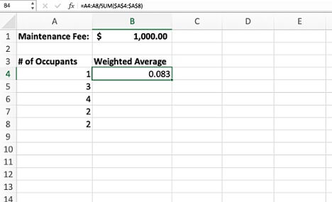Since one formula is designed to output to one cell in this environment, Pre-Dynamic Excel cannot spill the results to cells B4:B8 and must decide what value to return in the cell where the formula was entered. Though the @ symbol is not seen, Excel uses silent implicit intersection in the background to return the value using the cell in the same row or column as the formula. 

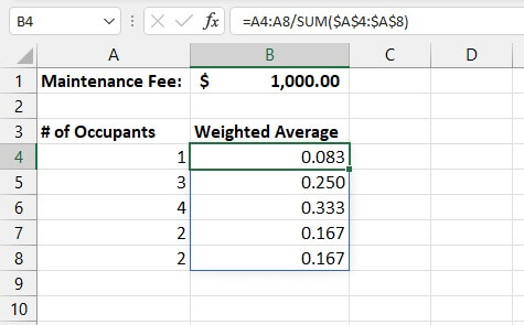
With the ability to return multiple values in Dynamic Excel, this same formula will spill results to the range B4:B8 automatically.

If you want to force Excel to return a single input, manually enter the implicit intersection operator, @, and Excel will use the value in the corresponding row to perform the calculation.

For example, in the image below, the H3:I6 array uses the SORT function to sort Region Sales from high to low instead of alphabetically.

=SORT(E3:F6,2,-1)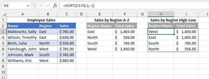

However, if we were only interested in knowing the name of the top sales region, we could place the implicit operator before the function name, forcing Excel to return a single value.

=@SORT(E3:F6,2,-1)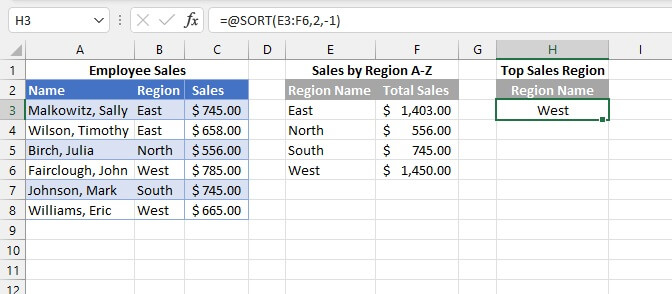

As the transition to Dynamic Excel continues, you may also see the implicit intersection operator for backward compatibility. When a formula that triggers implicit intersection is created in Pre-Dynamic Excel and is subsequently opened within the Dynamic environment, the @ operator may now be visible to indicate why only a single value has been returned.

Dynamic array functions & formulas       

There are eight new dynamic array functions that come with dynamic array characteristics built-in, meaning these functions are built to return dynamic ranges. These functions are:

• FILTER - filter records using criteria.
• RANDARRAY - generate a random list or array of numbers.
• SEQUENCE - generate a sequential list or array of numbers.
• SORT - sort a list or array by a column or row within that array.
• SORTBY - sort list or array by another list or array.
• UNIQUE - extract unique values from a list.
• XLOOKUP - flexible lookup returning corresponding values in a list or array.
• XMATCH - flexible lookup returning relative position of values in a list or array.

Combining dynamic array functions

The above functions are powerful on their own, but combining them allows you to accomplish multiple tasks in one entry. A few examples are shown below.

Example 1 - SORT and FILTER

SORT(array, [sort_index], [sort_order], [by_col])

FILTER(array, include, [if_empty])

With this combination, the SORT function is wrapped around the FILTER function to sort the results of a filtered array.

=SORT(FILTER(A2:D12,B2:B12="sandwich"),4)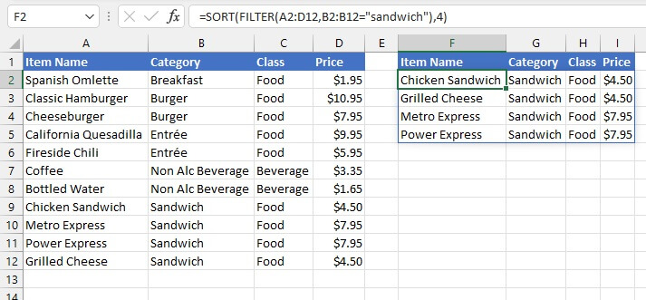

The formula in cell F2 filters the array A2:D12 by looking for records with the “sandwich” category. The SORT function sorts this array by price, the 4th column.

Example 2 - SORT and UNIQUE

SORT(array, [sort_index], [sort_order], [by_col])

UNIQUE(array, [by_col], [exactly_once])

Use SORT around the UNIQUE function to extract unique values within an array and then sort records that match a certain criterion.

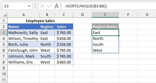The UNIQUE function above returns the distinct values in the B3:B8 range, and the SORT function was used to sort them alphabetically. The results were automatically spilled in the range E3:E6.

There are other options for the UNIQUE and SORT functions. 

Example 3 - COUNTA and UNIQUE

COUNTA(value1, [value2]…)

UNIQUE(array, [by_col], [exactly_once])

When COUNTA is nested with UNIQUE, you can quickly count the number of unique values in an array using a single entry.

=COUNTA(UNIQUE(Database[Team Name]))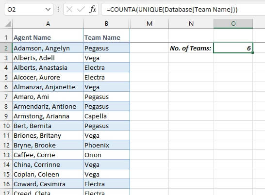

Example 4 - FILTER and FILTER

FILTER(array, include, [if_empty])

You can even nest a FILTER function within another FILTER to return selected columns of filtered records!

=FILTER(FILTER(Menu,Menu[Price]<5),{1,0,1})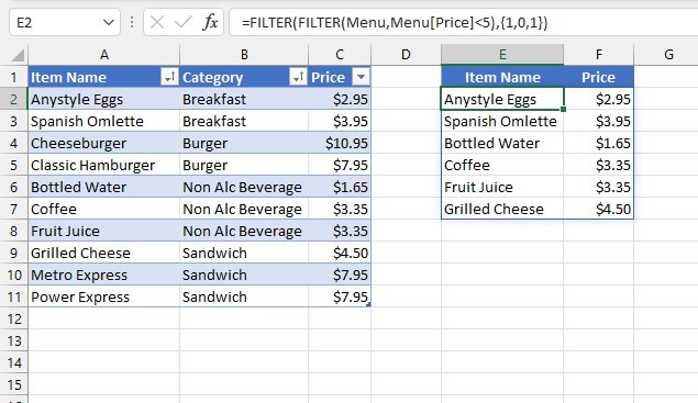

Using the array constant {1,0,1} as the include argument of the outer FILTER function tells Excel to exclude the 2nd column (since 1=TRUE and 0=FALSE).

Dynamic array data validation lists

In the old days, creating a dynamic dropdown list for data validation was an intermediate-to-advanced task because Excel did not have a built-in method to handle this. We would have needed to insert the new item somewhere in the middle of the source list or use the OFFSET function in combination with COUNTA to be able to add new items to the end of the source list. This was a fairly complicated solution.

Once the source list is created with a dynamic function or formula, creating a dynamic data validation list from a spilled array is now as simple as using the spill range indicator.

Step 1 - Create a source list using a dynamic array function or formula

In the example below, the SORT function was used to create an alphabetic source list.

=SORT(Menu[Item Name])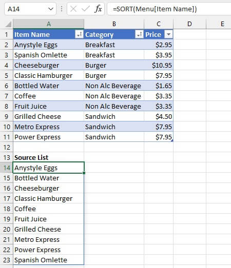

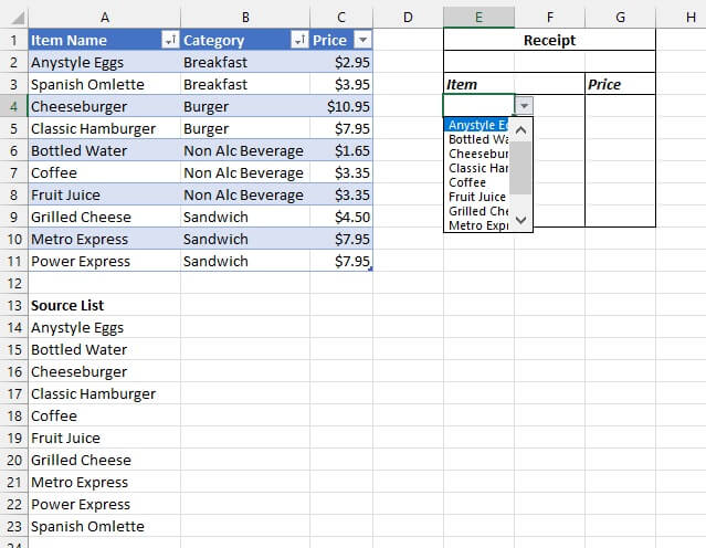
Step 2 - Use the spill range indicator to refer to the dynamic output

• From the cell where the dropdown list is desired, go to the Data tab and select the Data Validation command. Choose List from the Allow dropdown. 
• Refer to the spill range in the Source field. The spill range indicator must be manually entered after the reference to the first cell in the spill range. If the data validation will be copied to other cells, absolute cell referencing should be used.

=$A$14#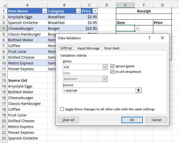

Errors when using dynamic arrays

In working with dynamic array formulas, you might encounter some new Excel error messages. Instead of getting bent out of shape about them, here’s a quick list of the more common ones and the possible causes.

• #SPILL! error

Message: Spill range isn’t blank

Excel will return a #SPILL! error message in the first cell of the spill range if there is an obstruction, that is, if any of the cells in the required output area is not empty. To correct this, clear the value(s) in the obstructing cell(s) or move the formula to a location that has enough blank cells to accommodate the output.

Message: Spill range is unknown

This error may occur when Excel cannot determine how many rows and columns will be needed for the output. For example, when volatile functions which return different values each time formulas are recalculated (e.g., RAND, RANDBETWEEN, RANDARRAY) are nested with certain other dynamic functions. See example below.

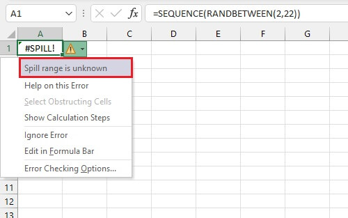Note that the same formula may work in some iterations and fail in others simply because of function volatility. You can either try again or calculate the formula step by step, i.e., generate the random values using the formula, copy and paste them as values, then manually place them in an array.

Message: Spill range in table

Somewhat surprisingly, Excel tables do not support spilled behavior at this time. This is most obvious when attempting to use one of the eight new functions where dynamic array functionality comes built-in. To use these functions, convert your Excel table to a range. For legacy functions, table behavior in Dynamic and Pre-Dynamic Excel are identical.

• #CALC! error

Message: Empty arrays are not supported

Since Dynamic Excel does not support empty arrays, any formula that results in an empty array will return the #CALC! error. For example, if no records in the source array match the criteria in the include argument of the FILTER function, Excel will return a #CALC! error. In that case, the solution would be to include the optional if_empty argument to display an alternative response. 

• You can’t change part of an array 

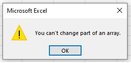This message comes in a popup window if you attempt to sort items in a spill range using the Sort command from the ribbon or contextual menu. 

This is because of the familiar principle that we cannot change part of an array formula (similar to the old CSE formulas). To sort a spill range, use the SORT function around the formula which created the spill range, for example:

=SORT(FILTER(A2:D12,B2:B12="sandwich"),4)

 (as illustrated in examples 1 and 2 above).

The way forward

Excited yet? Dynamic Excel represents a significant upgrade to the way in which formulas are processed in Excel. Eventually, pre-dynamic Excel will be a thing of the past, and dynamic arrays will be standard.

To learn more about using dynamic arrays in Excel, try our Microsoft Excel - Basic and Advanced course today.

Ready to become a certified Excel ninja?

Start learning for free with GoSkills courses

Start free trial