
About this article
In this detailed listicle, Alan Murray (a Microsoft Excel MVP) reduces choice overload by highlighting 12 useful Excel functions for data analysis for you to get started with. The article provides a free exercise file to follow along and links to resources to dig deeper. Some popular formulas covered that might interest you include:
There are over 475 functions in Excel. This can make it overwhelming when you are getting started with data analysis.
With such a large variety of functions, it can be difficult to know which one to use for specific Excel tasks.
The most useful Excel functions are those that make the task seem easy. And the good news is that most Excel users have a toolkit of just a few functions that complete most of their needs.
This resource covers the 12 most useful Excel functions for data analysis. These functions provide you with the tools to handle the majority of your Excel data analysis tasks.
Download your free practice workbook
Don't forget to download the exercise file to help you follow along with this article and learn the best functions for data analysis.
Learn the most useful Excel functions
Download your FREE exercise file to follow along
1. IF
The IF function is extremely useful. This function means we can automate decision making in our spreadsheets.
With IF, we could get Excel to perform a different calculation or display a different value dependent on the outcome of a logical test (a decision).
The IF function asks you for the logical test to perform, what action to take if the test is true, and the alternative action if the result of the test is false.
=IF(logical test, value if true, value if false)
In this example, we have displayed the word “Yes” if the delivery date in column C is more than 7 days later than the order date in column B. Otherwise, the word “No” is displayed.
=IF(D2>7,"Yes","no")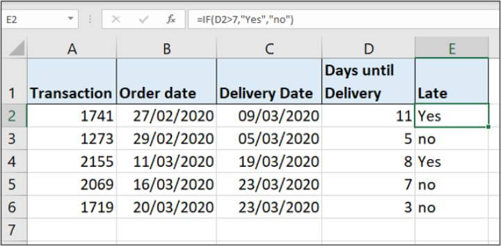
2. SUMIFS
SUMIFS is one of the most useful Excel functions. It sums values that meet specified criteria.
Excel also has a function named SUMIF which does the same task except it can only test one condition, while SUMIFS can test many.
So you can essentially ignore SUMIF as SUMIFS is a superior function.
The function asks you for the range of values to sum, and then each range to test and what criteria to test it for.
=SUMIFS(sum range, criteria range 1, criteria 1, …)
In this example, we are summing the values in column C for the region entered into cell E3.
=SUMIFS(C2:C9,B2:B9,E3)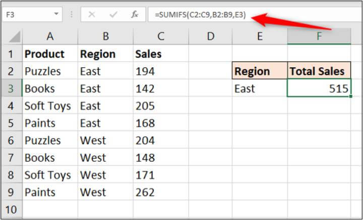
It is definitely worth exploring the SUMIFS function in more detail. It is an extremely useful Excel function.
3. COUNTIFS
The COUNTIFS function is another mega function for Excel data analysis.
It is very similar to the SUMIFS function. And although not mentioned as part of the 12 most useful Excel functions for data analysis, there are also AVERAGEIFS, MAXIFS, and MINIFS functions.
The COUNTIFS function will count the number of values that meet specified criteria. It, therefore, does not require a sum range like SUMIFS.
=COUNTIFS(criteria range 1, criteria 1, …)
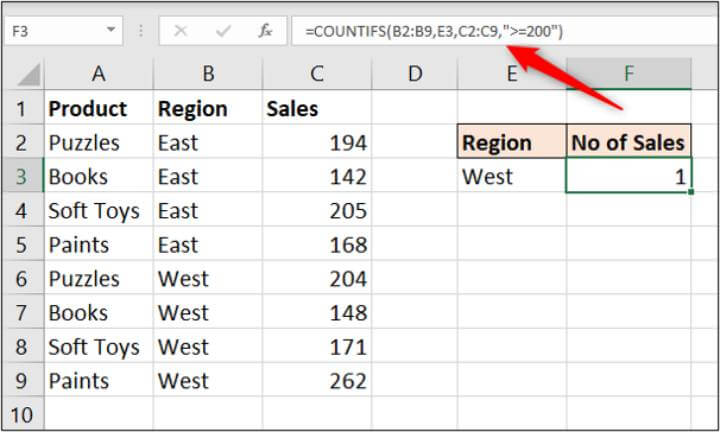
In this example, we count the number of sales from the region entered into cell E3 that have a value of 200 or more.
=COUNTIFS(B2:B9,E3,C2:C9,">=200”)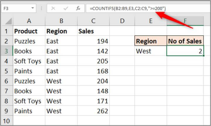
When using the SUMIFS and COUNTIFS functions, the criteria must be entered as text or as a cell reference. This example uses both techniques in the same formula.
4. TRIM
This brilliant function will remove all spaces from a cell except the single spaces between words.
The most common use of this function is to remove trailing spaces. This commonly occurs when content is pasted from somewhere else or when users accidentally type spaces at the end of text.
In this example, the COUNTIFS function from before is not working because a space has been accidentally used at the end of cell B6.
Users cannot see this space, which means it is not identified until something stops working.
The TRIM function will prompt you for the text to remove spaces from.
=TRIM(text)
In this example, the TRIM function is used in a separate column to clean the data in the region column ready for analysis.
=TRIM(B2)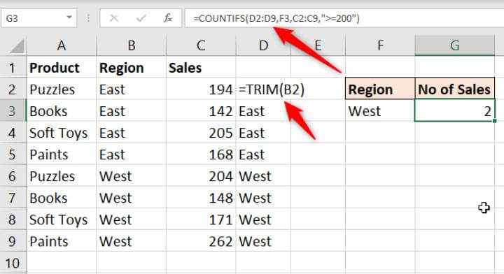
The COUNTIFS function then has clean data and works correctly.
5. CONCATENATE
The CONCATENATE function combines the values from multiple cells into one.
This is useful for piecing together the different parts of text such as someone's name, an address, a reference number or a file path or URL.
It prompts you for the different values to use.
=CONCATENATE(text1, text2, text3, …)
In this example, CONCATENATE is used to combine the firstname and lastname into a fullname. A space is entered for the text2 argument.
=CONCATENATE(A2," ",B2)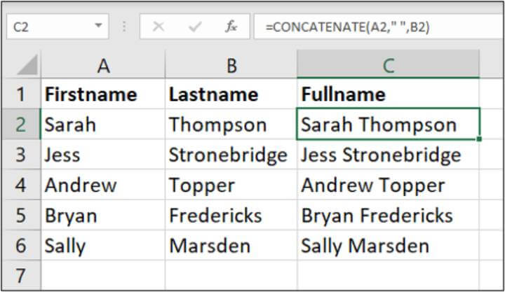
6. LEFT/RIGHT
The LEFT and RIGHT functions will do the opposing action of CONCATENATE. They will extract a specified number of characters from the start and end of text.
This can be used to extract parts of an address, URL, or reference for further analysis.
The LEFT and RIGHT functions request the same information. They want to know where the text is and how many characters you want to extract.
=LEFT(text, num chars)
=RIGHT(text, num chars)
In this example, column A contains a reference that is made up of the client ID (first two characters), a transaction ID, and then the region code (final character).
The following LEFT function is used to extract the client ID.
=LEFT(A2,2)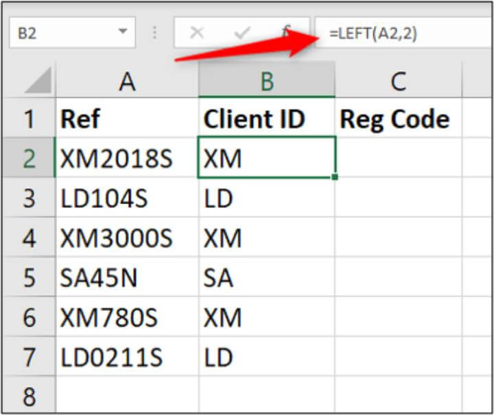
The RIGHT function can be used to extract the last character from the cells in column A. This example indicates whether the client is in the South or the North.
=RIGHT(A2,1)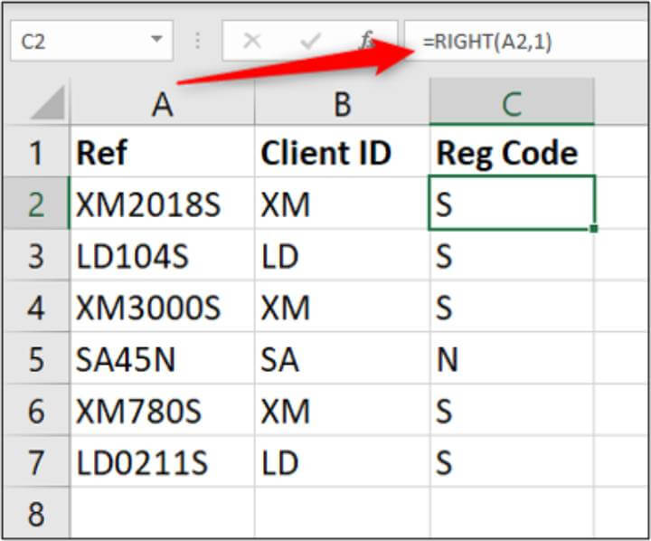
7. VLOOKUP
The VLOOKUP function is one of the most commonly used and recognizable functions in Excel.
It will look for a value in a table and return information from another column relating to that value.
It is great for combining data from different lists into one or comparing two lists for matching or missing items. It is an important tool in Excel data analysis.
It prompts for four pieces of information:
- The value you want to look for
- Which table to look in
- Which column has the information you want to return
- What type of lookup you would like to perform.
=VLOOKUP(lookup value, table array, column index number, range lookup)
In this example, we have a table containing sales from our employees. There is another table with further information about these employees (tables are kept small for the example).
We would like to bring the data showing which region the employee is based into the sales table for analysis.
The following formula is used in column D:
=VLOOKUP(B2,$G$2:$H$12,2,FALSE)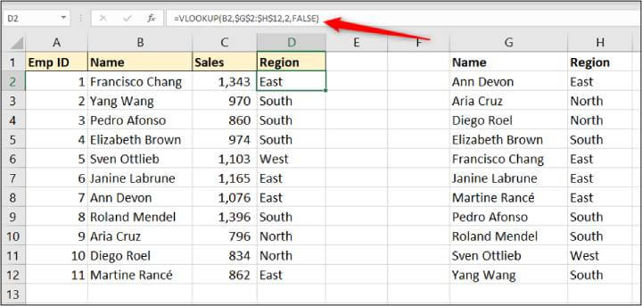
This can be one of the more difficult functions to learn for beginners to Excel formulas. You can learn VLOOKUP more in-depth in this article, or from our comprehensive Excel course.
8. IFERROR
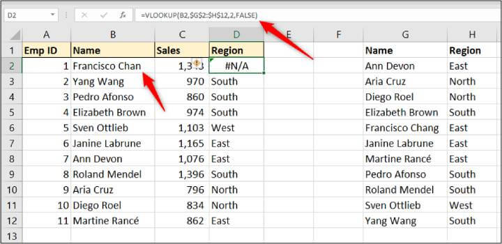
Sometimes errors happen that may be innocent and sometimes these errors may be things you can predict. The VLOOKUP function from before is a typical example of this.
We have an error because there is a typo in the name in the sales table. This means that VLOOKUP cannot find that name and produces an error.
Using IFERROR we could display a more meaningful error than the one Excel provides, or even perform a different calculation.
The IFERROR function requires two things. The value to check for the error and what action to perform instead.
In this example, we wrap the IFERROR function around VLOOKUP to display a more meaningful message.
=IFERROR(VLOOKUP(B2,$G$2:$H$12,2,FALSE),"Name not found. Check both lists")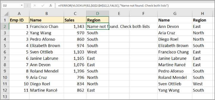
9. VALUE
Often the set of data you need to analyze has been imported from another system or copied and pasted from somewhere.
This can often lead to data being in the wrong format, such as a number being stored as text. You cannot perform data analysis tasks such as SUM if Excel does not recognize them as a number.
Fortunately, the VALUE function is here to help. Its job is to convert numbers stored as text to numbers.
The function prompts for the text to convert.
=VALUE(text)
In this example, the following formula converts the sales values stored as text in column B to a number.
=VALUE(B2)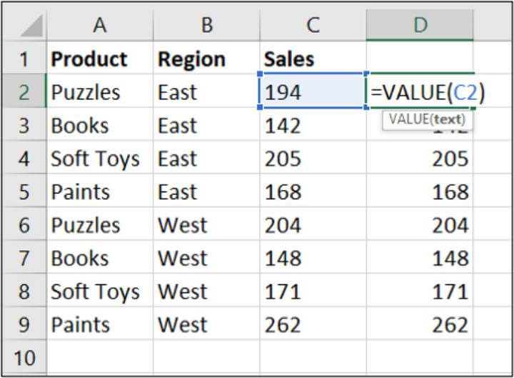
10. UNIQUE
The UNIQUE function is available only in Excel's dynamic array environment, that is, in Excel 365, Excel online, and Excel 2021 or later.
The function wants to know three things:
- The range to return the unique list from
- Whether you would like to check for unique values by column or by row
- Whether you want a unique list, or a distinct list (items that occur only once).
=UNIQUE(array, by col, exactly once)
In this example, we have a list of product sales and we want to extract a unique list of the product names. For this, we only need to provide the range.
=UNIQUE(B2:B15)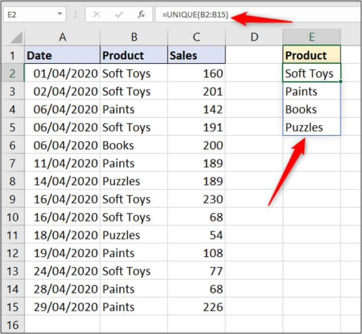
This is a dynamic array function and, therefore, spills the results. The blue border indicates the spilled range.
We can then use the SUMIFS function, mentioned earlier in this article, to sum the sales for each of those products.
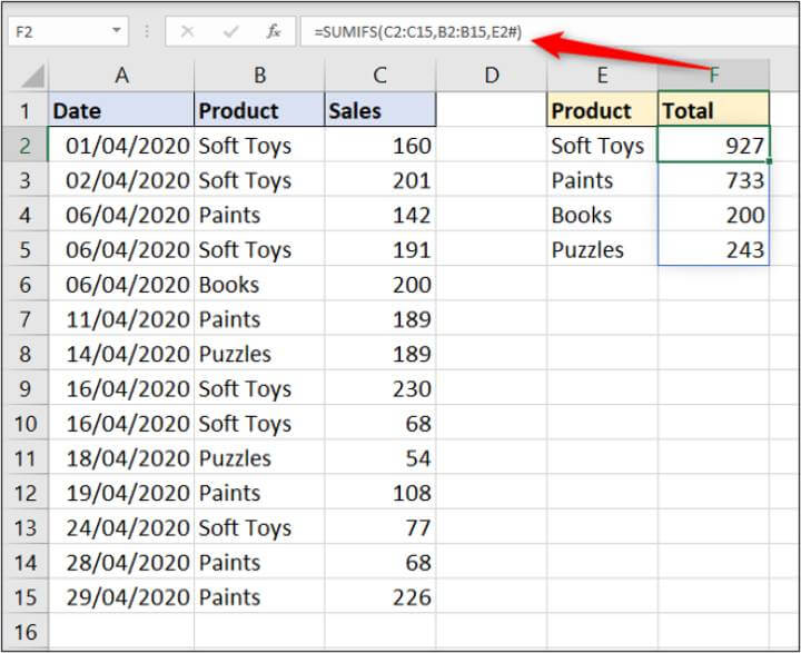
This should look familiar to earlier. However, a # was used to reference the spilled range this time.
11. SORT
This is another dynamic array function. As the name suggests, it will sort a list.
The SORT function prompts for four arguments:
- The range to sort
- Which column to sort the range by
- What order to sort the range (ascending or descending)
- Whether to sort the rows or the columns.
=SORT(array, sort index,sort order, by col)
This is fantastic. And it can be used with the previous UNIQUE example to sort the product names in order.
For this, we only need to provide it with the range to sort.
=SORT(UNIQUE(B2:B15))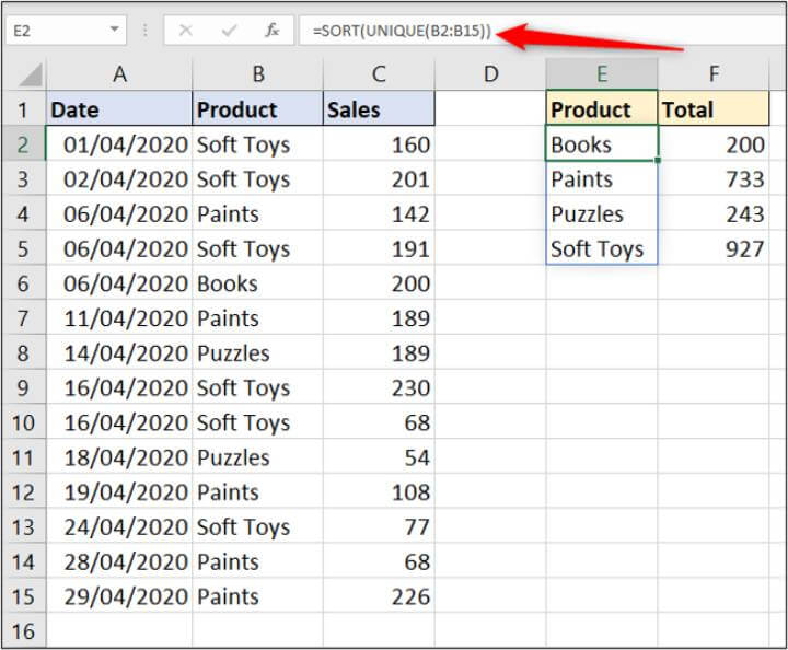
12. FILTER
Following the SORT function, there is also a dynamic array function to filter a list or range. This function will filter a range. It is an extremely powerful function and is a dream for analyzing data and producing reports.
The FILTER function takes three arguments:
- The range to filter
- The criteria that specifies which results to return
- What action to take if no results are returned.
=FILTER(array, include, if empty)
In this example, only the results for the subject entered in cell F2 are returned.
=FILTER(B2:C12,A2:A12=F2,"No scores")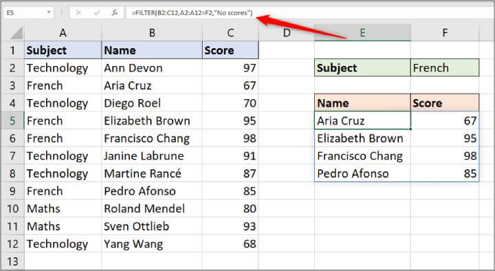
📌 Save this free cheat sheet with all 12 must-know Excel functions for data analysis we covered earlier — perfect for quick reference!

Wrap up
Learning the most useful Excel functions for data analysis mentioned in this article will go a long way to making Excel data analysis easier.
But there are still many more functions and Excel features to learn to be a true data analysis wizard.
Two other essential Excel tools to master are Power Query and Power Pivot.
Power Query makes importing and transforming data for analysis a breeze. And Power Pivot is the perfect tool if you analyze large volumes of data. It can store huge volumes of data outside Excel and has its own formula language called DAX.
Take the Power Query and Power Pivot courses on GoSkills to fast-track your data analysis skills in Excel today.