How to Use the COUNTIFS Excel Function

The COUNTIFS Excel function is especially useful when you want to count the number of cells that meet several criteria. As you probably guessed, it combines the functionality of the COUNT function with that of the IF function, much like the COUNTIF function. But COUNTIFS goes a step further with the addition of that letter — S.

By allowing the inclusion of multiple criteria, we can narrow down which cells qualify to be included in the count. Cells that are counted must satisfy all the criteria stated within the formula.

Syntax

The syntax of COUNTIFS is as follows:

=COUNTIFS(criteria_range1, criteria1, [criteria_range2, criteria2]…)

Criteria_range1 is the first range that will be evaluated for the desired criterion.

Criteria1 is the criterion that will be associated with criteria_range1. Criteria1 can be in the form of a number, expression, cell reference, or text that defines which cells will be counted. 

Criteria_range2, criteria2, and all subsequent range and criteria pairs are optional. Up to 127 range and criteria pairs are allowed.

---

---

How to use COUNTIFS - basic example

Here is an example of how the COUNTIFS function works.

In the following data table, we want to determine how many cell phone sales were made by representatives from the South region.

=COUNTIFS(D2:D21, “Cell Phone”, C2:C21, “South”)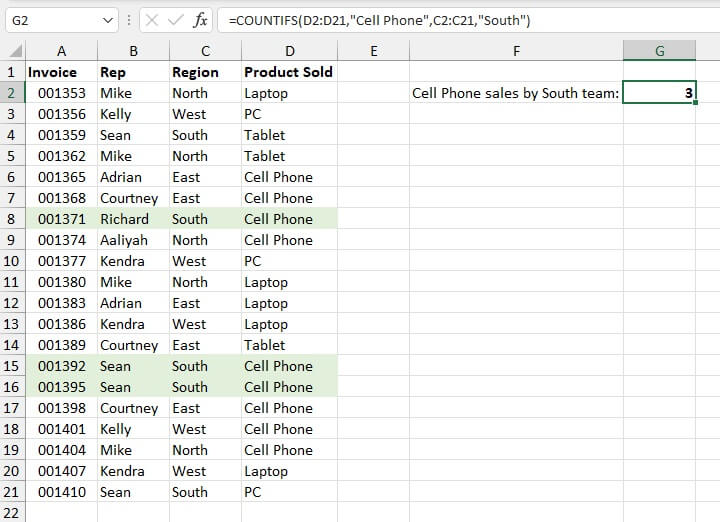

1. The first task is to identify occurrences of criteria1 (the text string “cell phone”) within criteria_range1 (the Product Sold range D2:D21). There are eight such occurrences.
2. Next, the formula looks within criteria_range2 (the Region range C2:C21) to determine how many instances of the text string “South” there are. There are five.
3. However, there are only three rows that satisfy both criteria, so the value 3 is returned as the result of our formula.

It can be seen from the above example that COUNTIFS uses AND logic, meaning all the stated criteria must be satisfied in order to be counted.

To count cells that satisfy at least one criterion (OR logic), we would use the COUNTIF function with the format:

=COUNTIF(range,criteria)+COUNTIF(range,criteria)

There are a few things worth pointing out in this basic application of the COUNTIFS function:

• Text strings are enclosed in double quotation marks.
• The COUNTIFS function is not case-sensitive. Therefore whether “South” or “south” was entered, the result would have been the same.
• When using text criteria, extra characters such as spaces within the double quotation marks will affect the results and give an incorrect count.
• There is no need to enter an equal sign (=) before the criteria value, as this is understood.

---

To count cells that satisfy at least one of many criteria, we would use the COUNTIF function.

---

Numeric criteria in COUNTIFS function

When a criterion comes in the form of numeric values, that value does not have to be enclosed within double quotes.

Below, we want to count how many Arts courses are being taught in Building 3. The formula is:

=COUNTIFS(B2:B18,“arts”,C2:C18,3)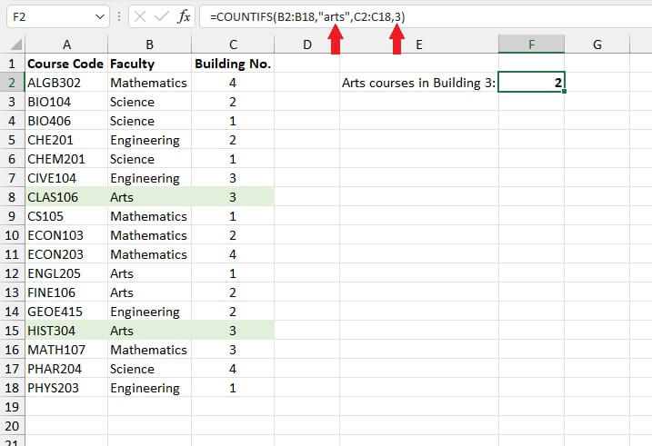

Note the differences in the way text criteria and numeric criteria are represented above.

Using cell references as criteria in COUNTIFS function

Criteria may also be entered using cell references. This offers the advantage of flexibility in the event that we want to change the values being counted. Instead of changing the formula because the criteria were hardcoded, the return value will update whenever we change the values entered in the input cell. 

For example, the formula below counts the number of laptop sales in the West region by using cells G2 and G3 as input cells for each criteria range.

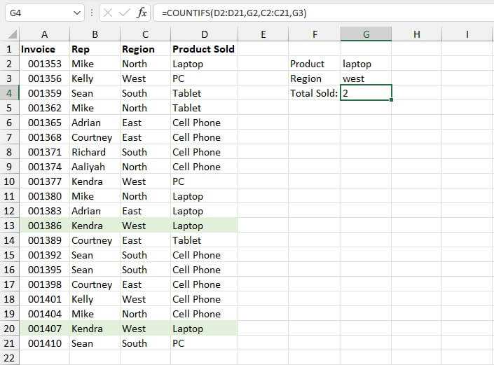We can quickly adjust what we want to count by entering different values in the input cells.

Note that when cell references are used as criteria, no double quotation marks are used because these (that is, “G2” and “G3”) are not the literal values being searched for.

Using COUNTIFS with logical criteria

COUNTIFS isn’t limited to counting exact matches. We can write our criteria to include cells that are greater than, less than, not equal to, or some variation of these with the use of logical operators (>, <). Logical operators such as >, <, = can be used to identify cells with values within a certain range. 

For example, the formula below can be used to count the number of sales made by a representative from the West region, which valued more than $400.

=COUNTIFS(C2:C21, “west”, E2:E21, “>400”)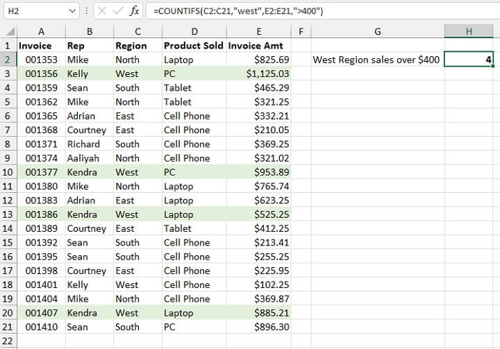

In this case, the entire logical expression is wrapped in double quotation marks. An alternative that yields the same result would be to write the formula as follows

=COUNTIFS(C2:C21, “west”, E2:E21, “>”&400)

where the concatenation operator (&) is used to join the greater than operator (>) to the lower limit value (400).

Similar formats are followed for criteria where values are greater than or equal to (>=), less than (<), or less than or equal to (<=).

Values not equal to

COUNTIFS can also count the number of cells not equal to, or excluding, a certain value. For this type of criterion, the symbol <> is used.

The following formula counts the number of sales from the North region where the value in the range D2:D21 is not equal to cell phone.

=COUNTIFS(C2:C21, “north”, D2:D21, “<>cell phone”)

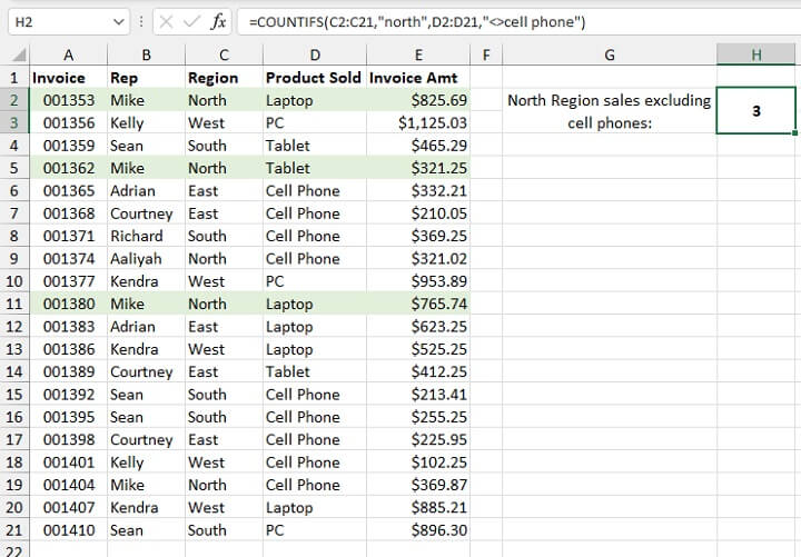As with the basic use of the COUNTIFS function shown earlier, if an extra space is entered within double quotes for text criteria, you will get an incorrect result since Excel is looking to match the text exactly.

However, if a space is entered between a logical operator and a numeric criterion, the correct value will be returned because Excel recognizes the value of the number. An example is shown below.

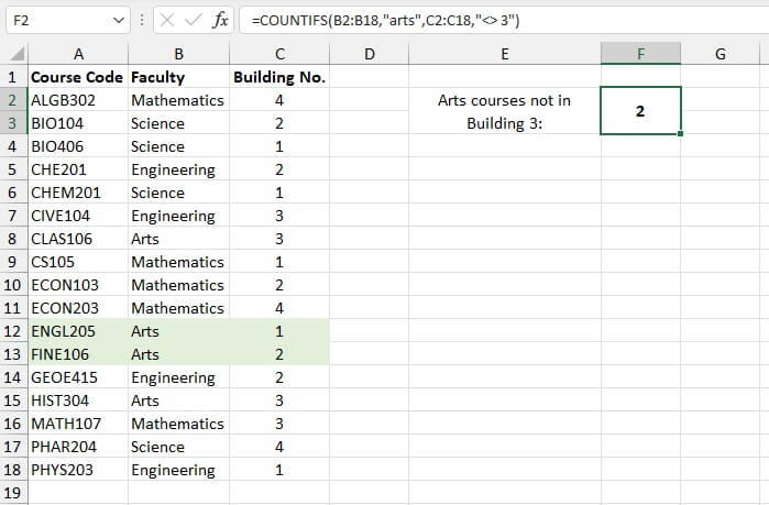Note that in the image above, there was a space entered between <> and 3, yet the formula returned the correct count. This principle also applies when the other logical symbols are used with numeric values.

Using logical operators with cell references

What about when logical operators are used with cell references? The format for that type of formula is worth remembering too. In the example below, cells G2 and G3 are our input cells. G2 is used to restrict the count to a particular date, and G3 is used as a lower-limit threshold.

=COUNTIFS(A2:A21,G2,D2:D21, “>=”&G3)

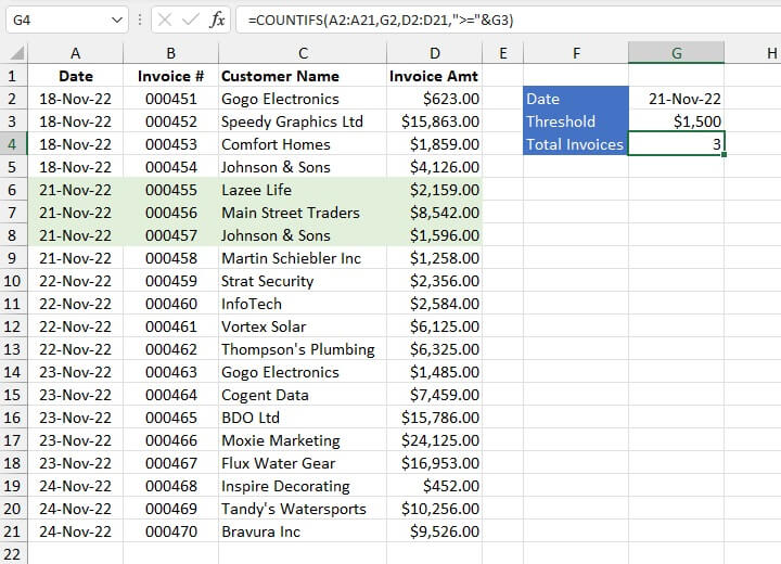Note that the double quotation marks are placed around the >= symbol, but not around the reference to cell G3. This is because “G3” is not the literal value being counted. The ampersand (&) is used to join the two parts of the expression.

Alternatively, the input cells could have been set up as below, and the formula written as follows:

=COUNTIFS(A2:A21,G2,D2:D21, G3)

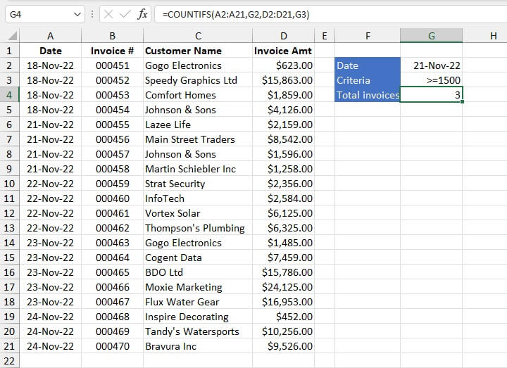In the above format, criteria2 is entered into the input cell rather than being hardcoded into the formula. The advantages of this method are: 

• It is easier to determine exactly what is being counted just by looking at our input cells.
• There are fewer formats to remember.
• There is greater flexibility when we want to change what is being counted. 
• There is less interference with our formula, which means that input errors are less likely.

Using COUNTIFS with a hardcoded date

If you prefer not to use a cell reference for a date in a COUNTIFS formula, you can hardcode the date within the formula using the DATE function.

=COUNTIFS(A2:A21,DATE(2022,11,21),D2:D21, “>=”&1500)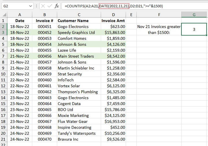

It is best not to use explicit dates such as “21-Nov-22” within the formula, as Excel may interpret them incorrectly and return an incorrect result.

Using COUNTIFS to count dates before or after

We can also use logical operators with dates to determine values that are before, after, or not equal to a certain date. 

The following formula counts the number of invoices issued before November 22, which were valued at $3000 or more.

=COUNTIFS(A2:A21, “<”&G2,D2:D21, “>=”&G3)

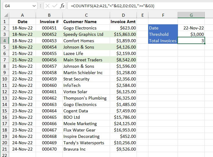Note that the “less than” symbol (<) is used to refer to dates earlier than the stated date, and the “greater than” symbol (>) refers to dates after.

COUNTIFS function with wildcards

A common problem when looking to summarize data is that the data we would like to count is often similar but not identical. Wildcards provide an excellent solution to this problem, and the COUNTIFS function does support the use of the following wildcards to accommodate partial matches. 

In the data set below, if we want to count the number of courses in the 100-series which are being conducted in Building 3, we would not be able to simply use the “100” as a text criterion since course codes are unique. We can use the asterisk (*) wildcard to represent the non-identical characters in our search criteria.

=COUNTIFS(A2:A18,"*1??",C2:C18,3)

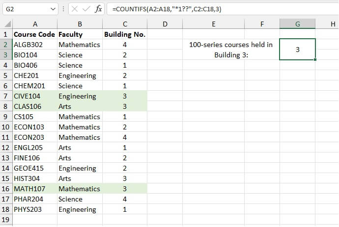The asterisk before “1” represents any number of characters before that text, while the two question marks represent exactly two characters after.

---

Wildcards are useful for identifying values that are similar but not necessarily identical.

---

Note that wildcards do not work with values stored as numbers. In the above example, our search for “*1??” worked because the values in the range A2:A18 are mixed with text. So Excel stores and treats the entire cell contents as text values.

Learn more about how to use wildcards here.

Using COUNTIFS with named ranges

Since the COUNTIFS function can accommodate up to 127 criteria/criteria_range pairs, it isn’t difficult to imagine that COUNTIFS formulas can get pretty difficult to build and read. By the time you get to the third pair, it is quite tedious to re-type ranges, and later, it may be quite challenging to quickly decode what each range refers to.

It is therefore often beneficial to define a custom name for ranges that will be frequently used.

The steps to create a named range are as follows:

1. Highlight a range that will be used frequently.
2. Type a descriptive name in the Name Box (e.g., Courses).
3. Press Enter.

A maximum of 255 characters are allowed in user-defined Excel names, and spaces are not permitted. Named ranges are valid on all sheets throughout the workbook.

Substituting named ranges where we previously had cell ranges results in a formula that is easier to construct and read. It has the additional benefit of eliminating the need for absolute references. 

=COUNTIFS(Courses,F2,Faculties,F3,Buildings,F4)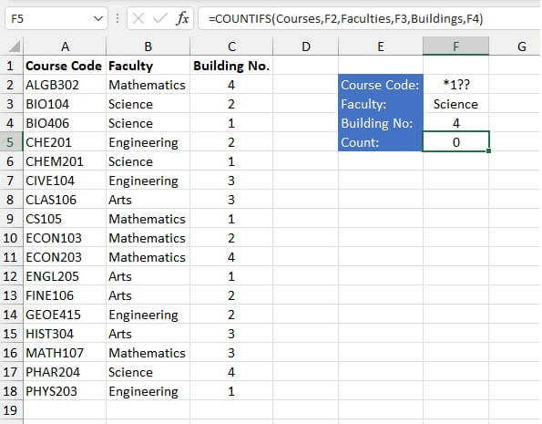

We have used the above COUNTIFS formula to count how many 100-series Science courses are taught in Building Number 4. The result is zero. The use of named ranges and cell references definitely makes this formula more readable.

COUNTIFS with non-contiguous ranges

Criteria_range arguments in COUNTIFS formulas do not have to be adjacent. They can begin and end in a different row and column, be on different worksheets, or even in another workbook, but the ranges must all have the same number of rows and columns. Otherwise, you will get a #VALUE error.

In the following example, the formula in cell F3 makes reference to two different data sets to determine how many classes a specified lecturer has in a particular building.

=COUNTIFS(H6:H22,F2,C2:C18,F3)

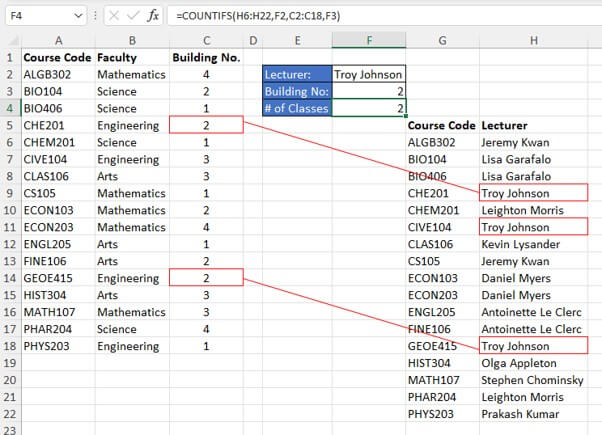Even though the name of each lecturer is in a different location on the worksheet, criteria_range1 carries the same dimensions as criteria_range2, so the formula in cell F3 returns a valid result. 

COUNTIFS determines the count by looking at each range for its respective criterion. If the corresponding position in each range satisfies that range’s criteria, that row’s position is counted.

Why we love it

The COUNTIFS function certainly takes away the need to create a pivot table or to try and figure out how to nest several functions into one formula to get the answer to a simple question. The syntax is easy to follow, and its compatibility with wildcards is a bonus. 

Try our Microsoft Excel - Basic and Advanced course to learn more useful Excel skills.

Level up your Excel skills

Become a certified Excel ninja with GoSkills bite-sized courses

Start free trial