The Ultimate Guide to Pivot Tables in Excel

When you have hundreds or even thousands of rows of data in Excel that need to be summarized or analyzed from different perspectives, few options work as well as pivot tables. Graphs and charts work best when data points are few, and formulas can be time-consuming to construct. 

What are pivot tables, and why do we use them?

So, what is a pivot table in Excel? The biggest clue is in the word “pivot.” Pivot tables are reporting powerhouses that give you incredible flexibility to change how data is summarized. With just a click here and a drag-and-drop there, you can modify the categories used to visualize, arrange, and analyze worksheet data.

Mastering pivot tables will reduce the time spent poring over worksheets, so you’ll have more time to actually take action on the data you're analyzing.

In this guide, we'll cover:

• How to create a pivot table
• Sort Pivot Tables by values
• Sort by totals
• Conditional formatting in Pivot Tables
• Pivot Table filters 
• Pivot Table slicers

How to create a pivot table in 5 steps

Pivot tables can handle complex data, but creating one doesn’t have to be complicated. In fact, in 5 simple steps, you can make a pivot table of your own. To illustrate how quickly and powerfully pivot tables can provide insight into large data sets from different angles, let’s use the following list of account subscribers to create your first pivot table.

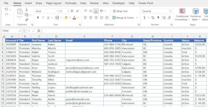
1. Make sure you have good data.

Good data is data with proper headers, consistent data types, accurate information, and no blank rows or unwanted duplicates. When entire rows are blank, this suggests to Excel that we have reached the end of the data set. When values are mistakenly duplicated, we may end up with incorrect results. You’ll also want to look out for numbers incorrectly formatted as text. In our case, some of our account holders have no phone numbers or no email addresses, but we have no rows that are completely empty.

2. Click the PivotTable command.

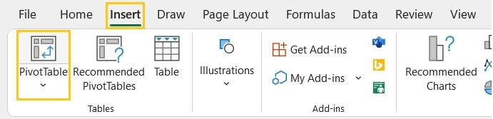
Click any cell within your source data, click the Insert tab on the Excel ribbon, and click PivotTable.

3. Fill out the PivotTable dialog box.

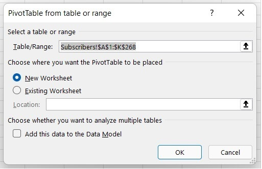
• ​Table/Range: field - Excel will usually select the range that contains the data to be summarized, but it doesn’t hurt to double-check. Make sure that the header row is included.
• New vs. Existing Worksheet - Your PivotTable can either be placed on the same worksheet as the source data or on a new tab within the same workbook.
• Add this data to the Data Model checkbox - Use this if you want to analyze multiple tables that have a relationship with each other. You will learn more about this when you start working with Power Pivot. For your first several PivotTables, you probably won’t need this option.

4. Decide how you want to summarize your data.

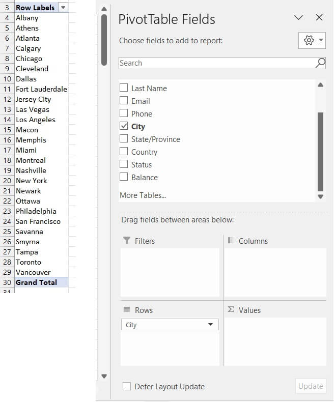
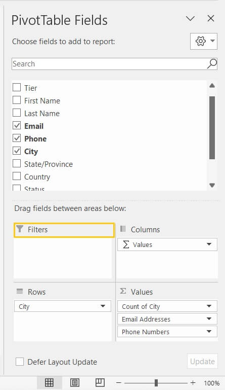
After the previous step, an empty Pivot table frame will appear within the worksheet, and to the extreme right, a pane listing the header names as possible fields to be added to the table.

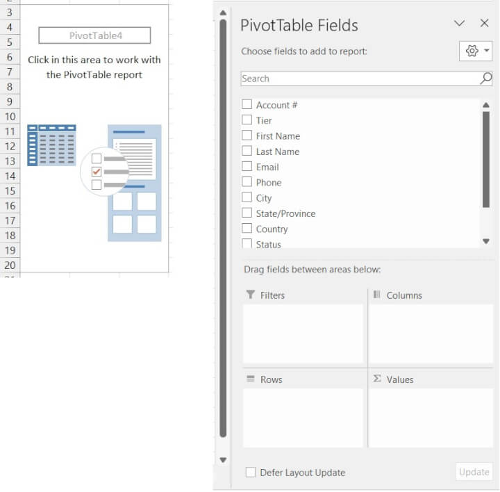
• Headers added to the Rows area will have each value in that category listed from top to bottom.
• Headers added to the Columns area will have each value within that category listed from left to right.
• Headers appearing in the ∑ Values area will be totaled, counted, averaged, or summarized in some other way as Excel sees fit. You can always change the summary method if you’re not happy with the one assigned.

If we drag the “City” header to the Rows area, we will see a list of all the cities in the dataset.

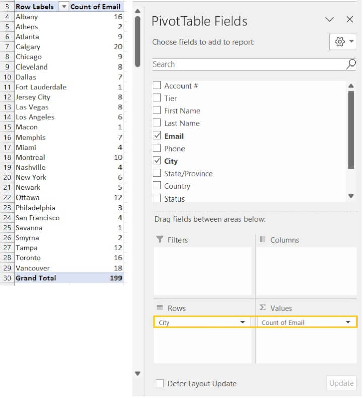
To find out how many email addresses we have for each city, drag and drop the “Email” header to the ∑ Values area.

5. Analyze and add/remove/change fields if desired.

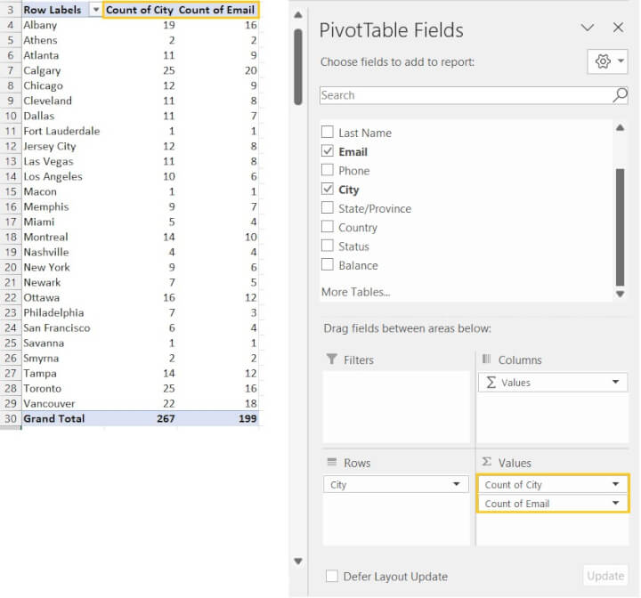
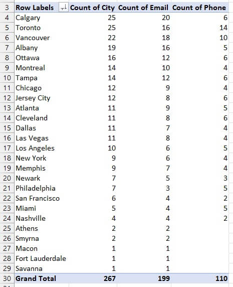
Now we know how many email addresses we have from each city, but how many subscribers do we have from each city? We can simply drag the “City” field to the ∑ Values area too.

Hot tip: The order in which the fields are stacked in each area will determine the order in which they appear in the pivot table. If we drag and drop the “Count of City” above “Count of Email”, the column containing the number of records for each city will appear before the “Count of Email” column.

​Sort pivot table by values

 

One of the simplest ways to organize data is by sorting. Sorting helps you find data quickly because they are listed in a logical order, which may be alphabetically, numerically, or in date order. You can sort a pivot table by its values rather easily.

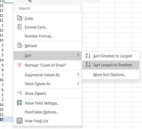
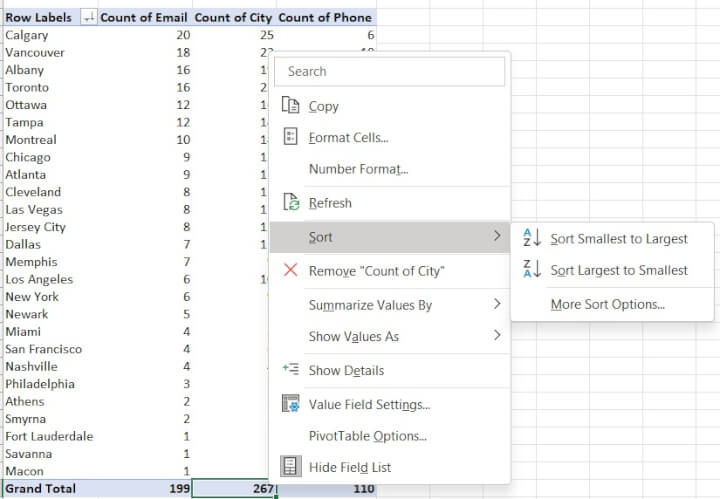
For instance, to display our list of cities from highest to lowest number of email addresses, we can right-click on a value in the “Count of Email” column, choose “Sort” from the contextual menu, then click the “Sort Largest to Smallest” option from the dropdown menu.​

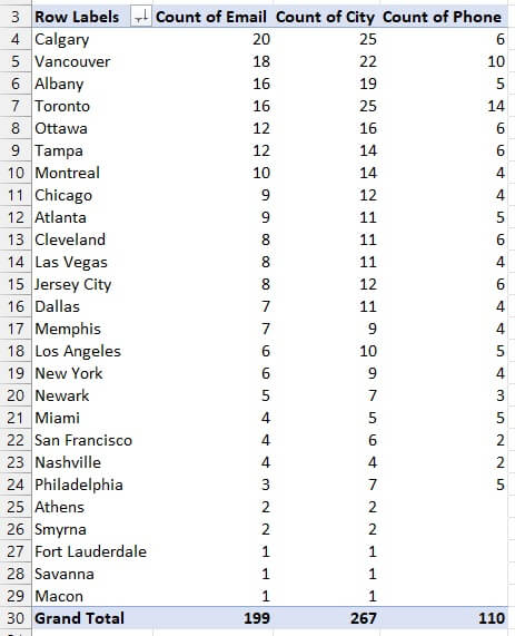
Our table is no longer organized by the name of the city, but by the number of records containing email addresses (Count of Email).

Sort by totals

To sort columns based on the value of the subtotal, right-click the subtotal row, click “Sort” from the contextual menu, and choose the sort order. The image below shows that there are 199 records with email addresses, 267 records with city names, and 110 records with phone numbers.

​If we right-click in the Grand Total row, we can make the columns rearrange themselves by the size of their totals.​

If we sort the totals from largest to smallest, then the ∑ Values columns will appear in the order: Count of City → Count of Email → Count of Phone.​

By doing this, we have essentially sorted the pivot table by totals from left to right.

Conditional formatting in pivot tables

Applying special formatting to cells based on their value or other conditions is a useful visual tool. 

Using conditional formatting in a pivot table is not very different from using it with any other data set within Excel. 

1. Select the cells to be analyzed 
2. Go to the Home tab, 
3. Look for the Conditional Formatting command. 

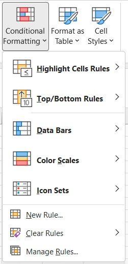
4. Choose the type of action you would like to perform and the rule to be applied. You can even create your own rule by clicking “New Rule…” if none of the built-in rules are suitable.

Pivot table filters

Filtering is a way of displaying only a specific subset from a larger set of data. There are a number of ways to filter pivot table data.

1. Apply Manually

Applying a manual filter is the most basic way to temporarily exclude certain data from a report. Go to the header row and select the filter drop-down arrow for the column you want to filter.​

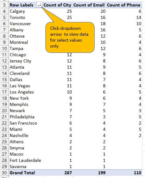Uncheck “Select All”, then select only the values you want to be displayed.

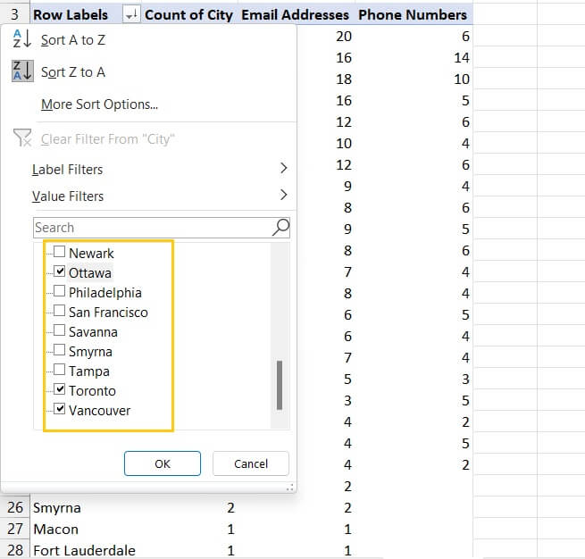
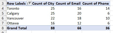
The pivot table will now display only the rows where the selected values appear in the filtered list. 

2. Using the Filters area of the PivotTable Fields pane

Another useful tool is the Filters area of the PivotTable Fields pane.

Another clever pivot table filter is the often-forgotten (sometimes unknown) slicer. 

Pivot table slicers

Excel slicers are similar to filters, but they’re a more interactive way of visually filtering elements within a table. Since pivot tables already narrow down data to display exactly what you want to see, pivot table slicers allow even more interactivity so that the data on the table is updated dynamically.

How to add a slicer to a pivot table

1. Click inside the pivot table.
2. Go to the Insert tab and click “Slicer” within the Filters command group.
3. Choose the category or categories containing the values you want to be able to hide or display.
4. Resize or move the slicer(s) to a location where you can easily view and manage your pivot table(s).

At first glance, slicers may seem like nothing more than glorified list filters, but don’t dismiss them just yet - they can even save you time by controlling the display of multiple pivot tables simultaneously.

Link a slicer to multiple pivot tables

You can create multiple pivot table slicer connections by doing the following:

1. Ensure that each pivot table was created using the same source data.
2. Add the slicer for the first pivot table as outlined in the previous paragraphs.
3. Click the slicer then go to Slicer tab > Report Connections.
4. Select the reports to be linked to that slicer. Click OK.

Take it to the next level

Ready for more? To practice creating pivot tables with another real-world example, try this case study.

Unlock even more by learning how to create calculated fields and other advanced pivot table techniques with our Microsoft Excel - Pivot Tables course.

Level up your Excel skills

Take the Pivot Tables course today!

Start free trial