How to Sort a Pivot Table

Did you know that you can sort pivot table data to present the items and values of your report in the correct order? The method for sorting pivot table data is very similar to how you sort data in an Excel table, but there are still a few differences that are important to know. 

In this a complete guide on how to sort a pivot table, we begin with the basics and then cover some lesser known techniques such as applying custom sort orders, manually sorting data and sorting values from left-to-right.

Download the sample workbook used in this guide to follow along.

How to sort a pivot table by row label

The simplest way to sort a pivot table is by using the field filter arrow in the header of the pivot tables row label.

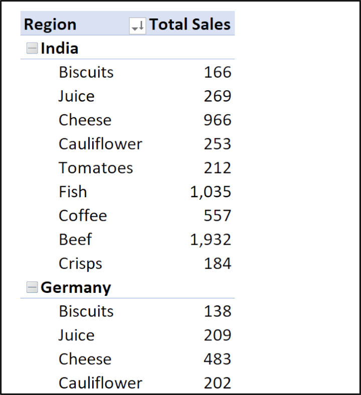
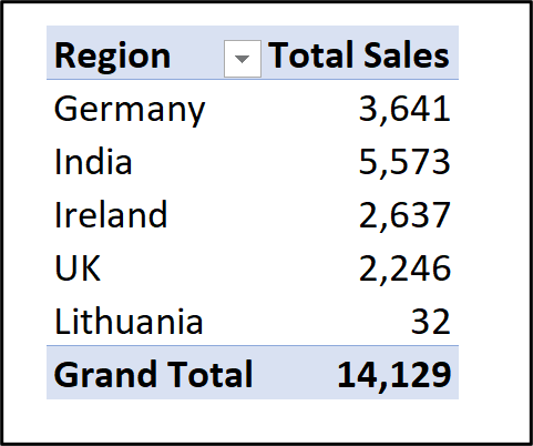
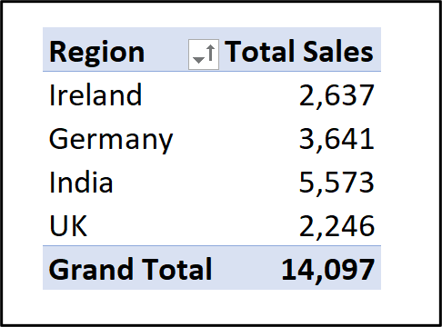
In the image below, the names of the countries are not in the desired order. As the country names are in the row labels area of the pivot table, a field filter arrow can be seen in the cell containing the word “Region.”

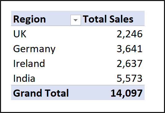
A filter arrow is not provided for the values of the pivot table, so we'll take a different approach to sorting them shortly.

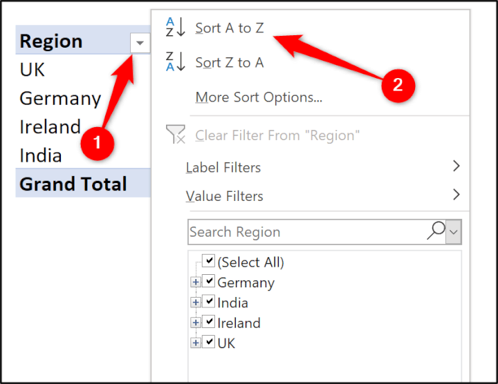
Click the field filter arrow and choose Sort A to Z to order the country names alphabetically.

Sort pivot table by values

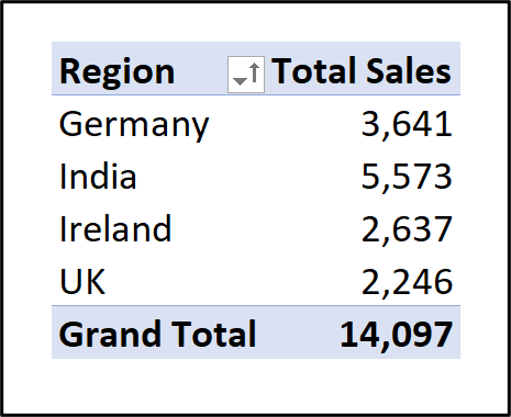
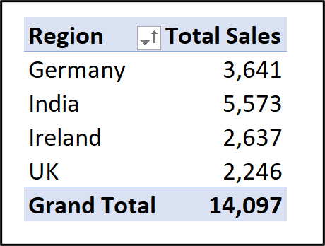
The image below shows the pivot table ordered alphabetically by country name from the previous sort, and no filter arrow in the cell containing the text ”Total Sales.”

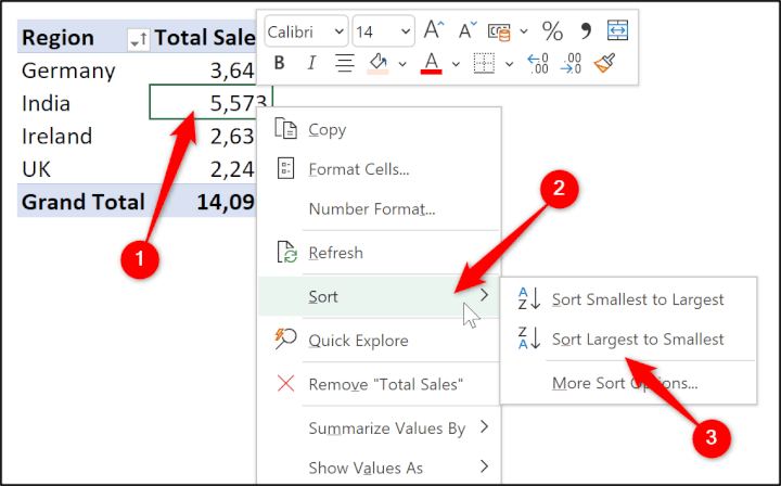
The easiest way to sort Pivot table values, is to use the right-click context menu.

Right-click on any value in the pivot table and select Sort Largest to Smallest to order the data with the larger total sales values first.

Sort on a column with multiple row labels 

When multiple fields are added to the row labels area of a pivot table, users are often mistaken in thinking that the filter arrow cannot be used to filter the second field.

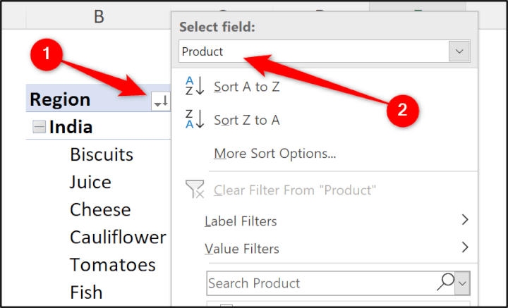
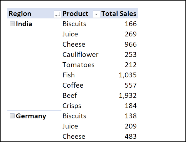
In the image below, the “Product” field has been added to the row labels area which already contained the “Region” field. There's only one filter arrow for that column.

To sort the pivot table by the product name in ascending order for each country, we could right-click any cell containing a product name and choose Sort A to Z. 

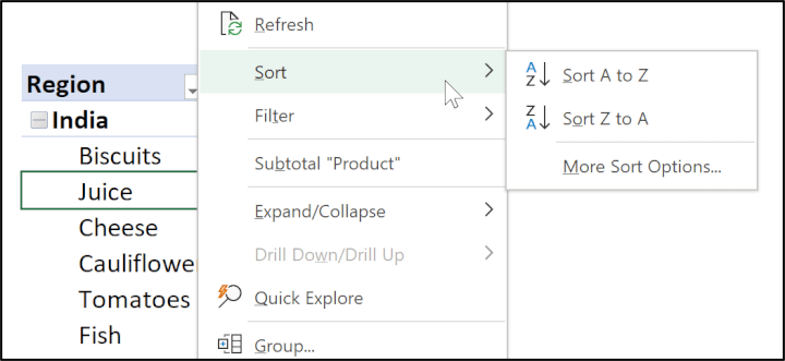
While that's a great approach, you can also sort the labels using the filter arrow, as there's an option to select the field to sort by country or product.

Click the filter arrow, click on the Select field list and choose “Product,” and then click Sort A to Z.

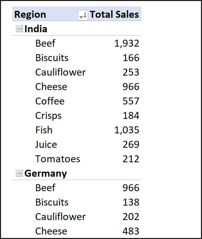
And there you have it! The product names are sorted alphabetically within each country. 

The confusion around a column not having an arrow button is caused by the default compact view of a pivot table. A pivot tables layout can be changed by clicking the Design tab of the pivot table followed by Report Layout.

In the image below, the pivot table is display in the tabular layout. In this layout, a filter arrow is shown for the column, and it can be sorted as shown in the first example.

Pivot table sort not working on refresh

When new records are added to the pivot table source data, and the pivot table is refreshed, the Pivot items are not always sorted immediately.

In this example, a new record has been added to the source table for the new country of “Lithuania.” On refreshing the pivot table the sort did not immediately apply.

If this occurs, the solution is to re-apply the sort to the pivot table labels using any of the previously discussed techniques.

It can also be the case that the pivot table sort by value is not working on refresh, and the solution would be the same.

This doesn't seem to occur as often in modern versions of Excel, but is still a problemto be aware of. 

Sort items in the pivot table’s report filter

Another area of a pivot table that may require sorting is the report filter. If you right-click the report filter cell, no sort functionality is provided. So how do we sort the report filter items?

In this case, we will add it to another area of the pivot table, sort the items, and then move it back to the report filter.

Manually sort pivot table data

You may be wondering what this means, or how to manually sort pivot table data. It seems like an unorthodox requirement. However, this has been the default setting in many Excel versions. Let’s look at how and why to adjust this setting.

The option to manually sort is one of the custom sort options for pivot tables, and this setting can prove useful to take control over the order of the items. Not all text values follow an A to Z order e.g., gold, silver, bronze or Spring, Summer, Autumn, Winter.

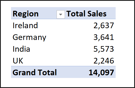
In the following pivot table, the “Region” field is used in the row labels area of the pivot table and are in a standard A to Z order.

Now, let’s imagine that Ireland is where we have our flagship store and head office. And therefore, we would always like to see Ireland first in any list, followed by the other regions in A-Z order.

Click on the field filter arrow for the row labels area and select More Sort Options.

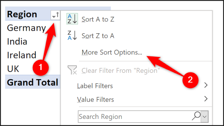
In the Sort Options window, click Manual and then click OK.

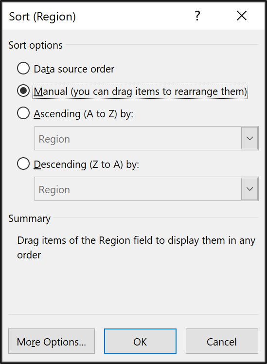
The items of the “Region” field can now be dragged into any order.

Click on a cell containing the region you want to move, and position your mouse cursor over the border of the active cell until you see the mouse arrow cursor change to the move cursor (four black arrows facing away from each other), and drag the region to the desired position.

In the following pivot table, the “Ireland” label has been dragged to the top of the row labels list.

You can only set manual sorting for label fields in a pivot table. If you check the sort options for a values field, manual sort is not there.

Sort a pivot table field left to right

Another interesting custom sort option for pivot tables is the ability to sort items from left to right.

Labels and values are typically sorted vertically, but if you are using the column labels area of a pivot table, you may have a need to sort horizontally. In the following pivot table, the “Region” field has been used in the column labels area of the pivot table.

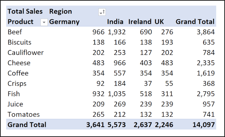
Let’s imagine that we want to sort the values for the “Product” of “crisps” in a largest to smallest order. Since the values are displayed along a row, we need to sort left to right.

1. Right-click on one of the “crisps” values.
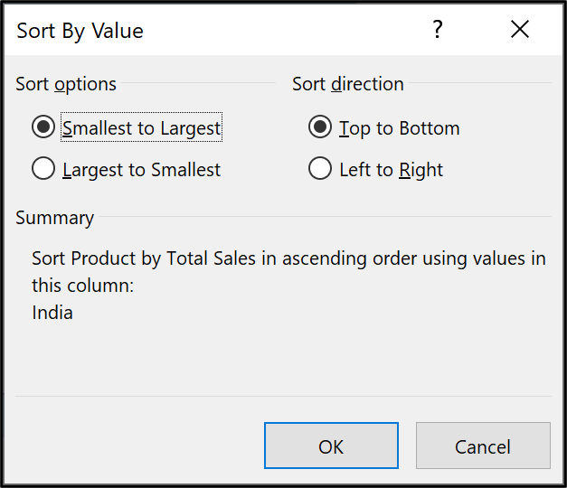
2. Position your mouse on the Sort option and click More Sort Options.
3. Click the Largest to Smallest option in the Sort options section of the window.
4. Click Left to Right in the Sort direction section of the window and select OK.

All values in the pivot table are now following the order of largest to smallest for the product “crisps.”

Interestingly, if you were to right-click on one of the grand total values and click Sort > Sort Largest to Smallest, they would naturally sort left to right without needing to specify this.

Set a custom order to sort pivot table labels

We saw how to manually sort pivot table labels earlier in this guide, but if this sort order is something you use regularly, and even use beyond the use of pivot tables, then creating a custom list would be a better option.

Custom lists exist in Excel to specify the sort and fill sequences for text values that are exempt from the A to Z order. By default, custom lists are already created for the order of days of the week and months of the calendar year. 

We should have no need to set custom sort options to enable custom lists for pivot tables, as it is set by default. So, when you add day of week or month labels to a pivot table, they should automatically appear in the correct order.

To view or change this setting:

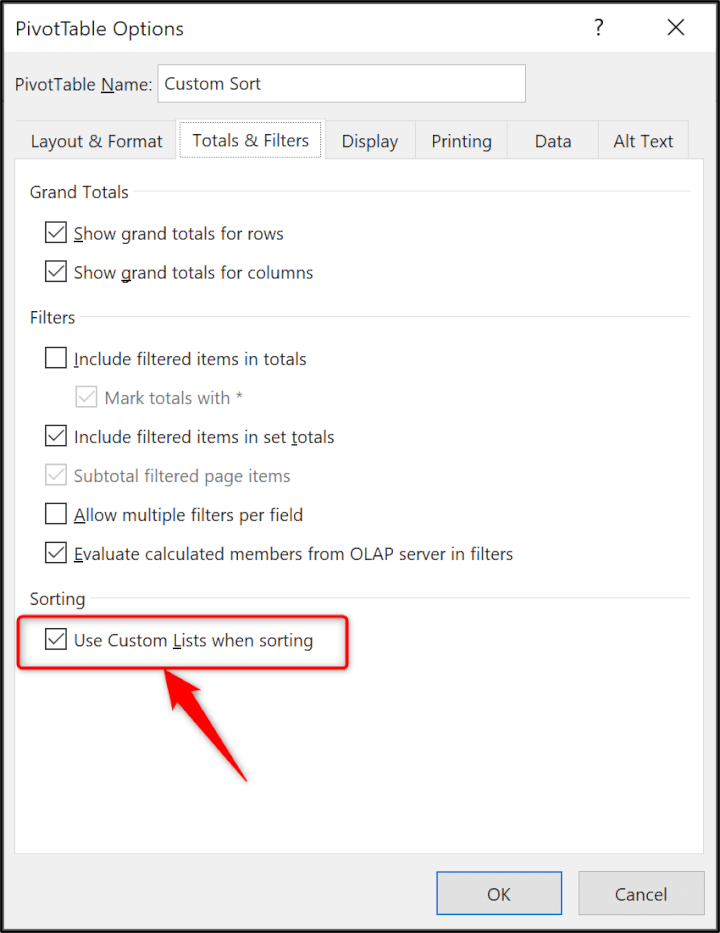
1. Click the pivot table Analyze tab and then the Options button in the pivot table group.
2. Click the Totals & Filters tabin the pivot table Options window.
3. The Use Custom Lists when sorting option is at the bottom of the window. In the following image you can see that the box is checked.

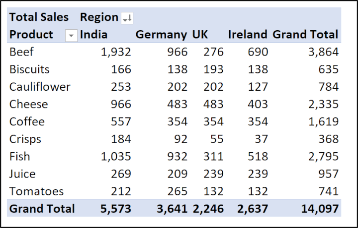
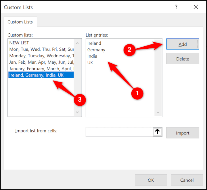
You can create your own custom lists. Let’s imagine we want to create a custom list for the order of the regions. We want to set the order to Ireland, Germany, India, UK to custom sort the pivot table labels in this order (and also have it available outside of pivot tables).

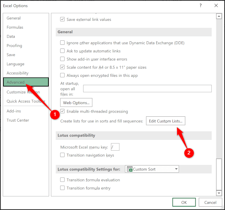
To view, create and edit custom lists in Excel:

1. Click File > Options > Advanced.
2. Scroll to the bottom of the Advanced category and click Edit Custom Lists.

3. In the Custom Lists window, Enter each region on a separate line in the List entries box and click Add (you can also add a list of entries from a range on a sheet). The list of regions will appear in the Custom lists box on the left. Click OK to each window.

The list of regions in the pivot table are not sorted immediately. You will need to apply the A to Z sort order. The items will then be order as per the custom sort order we defined with the custom list.

The image below shows the finished pivot table. The icon in the field filter arrow visualizes that the items are ordered A to Z, but the Use Custom Lists when sorting option overrides it.

 

Now that you’ve conquered how to sort pivot tables, perhaps it's time to challenge yourself with leveling up the rest of your Excel skills!. Check out our Basic and Advanced Excel course to become an Excel whiz in no time. 

Level up your Excel skills

Become a certified Excel ninja with GoSkills bite-sized courses

Start free trial