
What is the OR function?
The Excel OR function is a logical function that determines if at least one condition is true from multiple criteria. Even if only one condition is true, that value passes the test.
The syntax, or format, of the OR function is:
=OR(logical1, [logical2],...)The OR function can handle up to 255 arguments, each of which is a logical test. Only one argument is required. However, if you’re using an OR function it is likely you’ll have at least two.
How to use the Excel OR function
Download your free practice file
Use this free Excel file to follow along with the OR function tutorial.
Example 1
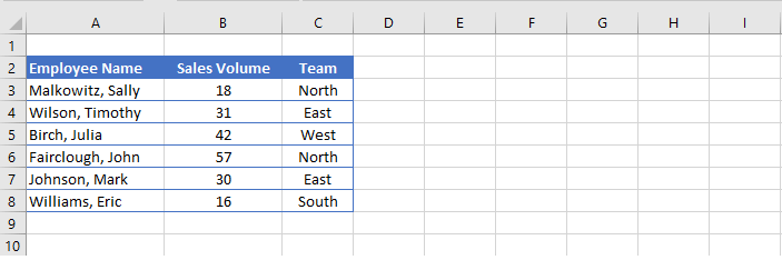
Here’s a practical example of how the OR function can be used. The Sales Department wants to reward all employees on the North team for outstanding overall performance, plus anyone with more than 30 sales from any other team. Either of these two conditions would qualify an employee for that reward.
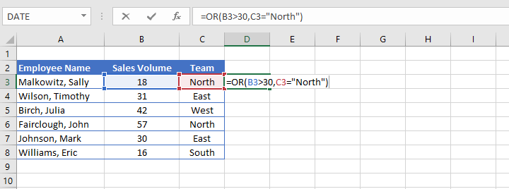
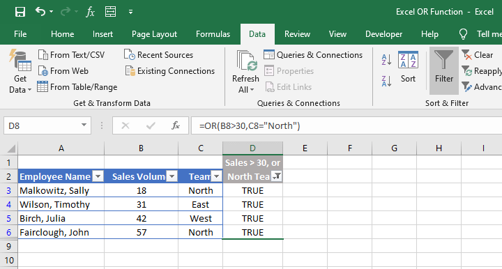
 In order to identify the rows which satisfy one or both criteria, two statements are required. The first statement would say that the value in cell B3 is greater than 30, and the second statement would say that the value in cell C3 is equal to the word “North”. The OR formula would read as follows:
=OR(B3>30,C3=“North”)
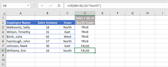
 If both statements are true, the result TRUE is displayed. If at least one statement is true, the result TRUE is displayed.
If neither statement is true, Excel returns a value of FALSE.
Use with the Filter feature
The OR function works well with the Filter feature because it is easy to display only the rows that satisfy at least one of the stated conditions and to hide those that don’t.
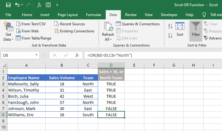 From the Data tab on the Ribbon, click on the Filter icon and use the filter arrows at the top of the dataset to select only the rows with TRUE values in column D. Click OK to apply the filter.
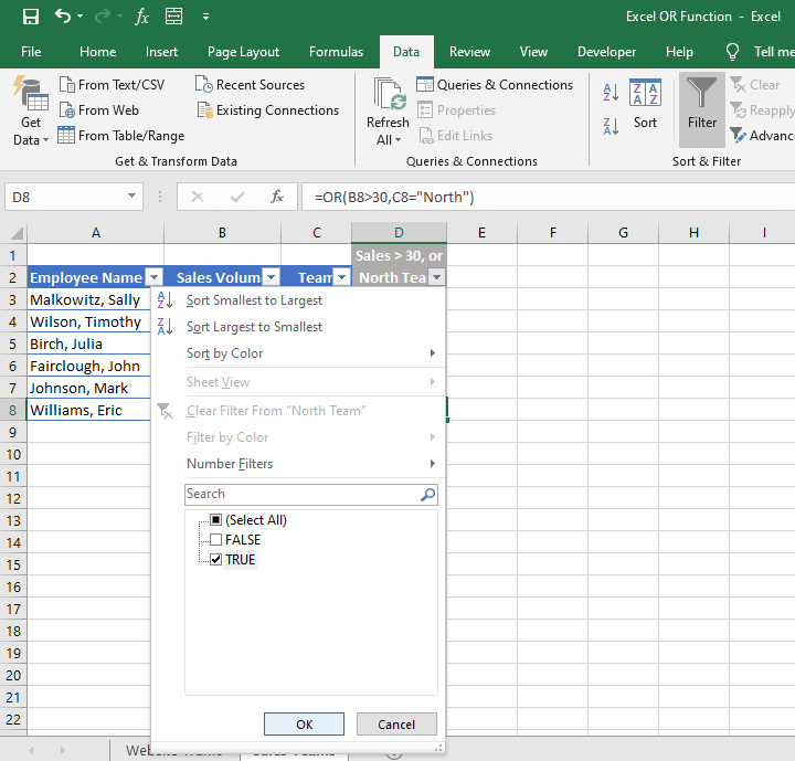 The rows which do not satisfy either one of the stated criteria are filtered out of the display, as indicated by the blue row numbers.
Use with the IF function
There are other ways to get creative with the OR function.
It’s often nested with the popular IF function to create a customized response instead of TRUE or FALSE.
Since the first argument of the IF function calls for a logical test, we can make the OR function itself the logical test.
We would type:
=IF(OR(B3>30,C3=“North”),The argument after =IF( above, which was the entire OR formula before, now becomes the first argument of the IF function.
Instead of the generic TRUE response, the second argument in the IF function allows a specific value or mathematical calculation to be entered if the previously-stated argument is true. Text values must be enclosed in double quotes, but numerical values and mathematical formulas are entered without double quotes.
A third argument may be entered for the IF function’s value_if_false. If no third argument is entered, a result of FALSE will be displayed for rows that fail both criteria.
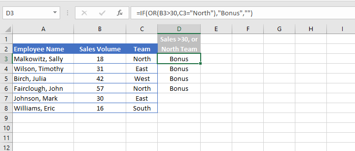
However, entering an empty pair of double quotes as the third argument for the value_if_false will result in blank cells for rows that fail all stated criteria.
The logical statement...
“If B3 is greater than 30, or if C3 is equal to “North”, then display the word “Bonus”. Otherwise, display a blank cell,”
...would be represented in Excel as follows:
=IF(OR(B3>30,C3=“North”),”Bonus”,“”)
 Example 2
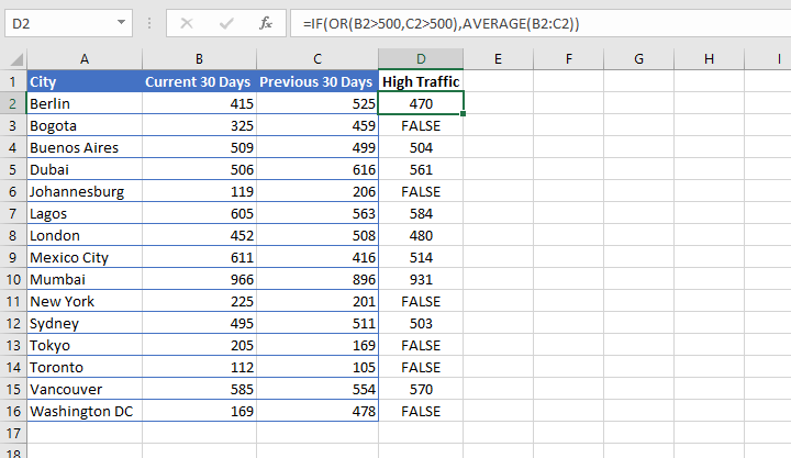
Here is an example of how to use the IF/OR combination with a mathematical calculation for the value_if_true. The following spreadsheet displays visits to a company’s website for the current 30-day period and the previous 30-day period.
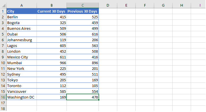 If either column B or column C has a value greater than 500, that is considered a high-traffic location.
We want to identify the cities which are high traffic locations and calculate the average number of visits for the two months on the report. If a city is not considered a high traffic city, no average should be calculated.
As in the previous example, the IF and OR functions would be nested for Argument 1 as follows:
=IF(OR(B2>500,C2>500)The second argument would take the form of the AVERAGE function:
AVERAGE(B2:C2)The third argument may be omitted to return a value of FALSE, indicating that those cells did not meet any of the given criteria.
The full formula would read:
=IF(OR(B2>500,C2>500),AVERAGE(B2:C2))The result of the worksheet when this formula is copied to all the relevant cells in column D would be:
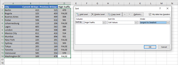
Use with sorting
The Sorting feature may now be applied to generate a high-to-low or low-to-high list of cities by traffic volume.
Summary
The Excel OR function is useful for performing tests within a single function to identify cells that meet any one of multiple criteria.
Because of its simplicity, the logic is easy to follow and it can be applied to virtually any type of dataset. Combining it with other functions and features of Microsoft Excel makes it both practical and versatile.
To learn more essential Excel functions and formulas, try our Microsoft Excel - Basic and Advanced course today. Or try the free Excel in an Hour crash course to cover some basics in Excel.