How to Use the Excel LEFT Function

---

When you want to extract some values from one location in Excel without copying all the cell’s contents, the Excel LEFT function might be just the thing you need. 

Purpose

LEFT is very useful when you only need a fragment of a longer piece of text. This function extracts a character or a specific number of characters from a text string, starting from the leftmost character. This function relies on the relative position of characters in a text string.

Return value

The value returned by the LEFT function is the character or characters in the original text string which meet the conditions stated in the formula.

Syntax

The syntax of the LEFT function is: 

LEFT(text, [num_chars])

Arguments

The text argument is the text string from which you want to extract characters. This may be entered as a text string within double quotes inside the formula itself, or (more commonly) it could refer to a cell reference that contains the characters to be extracted.

The num_chars argument is optional. It tells Excel how many characters you want to be copied from the original text string, starting with the first (leftmost) character. If num_chars is omitted, it is assumed that you only want the very first character.

For example: 

=LEFT(“apples and oranges”,5) will return the word apple.

=LEFT(“apples and oranges”) will return the letter a.

Remarks

• If num_chars is zero, LEFT will return an empty cell.
• If num_chars is not an integer, Excel will truncate the number and return the relevant characters.
• If num_chars is a negative number, LEFT will return a #VALUE! error.

So now you know how LEFT works, but can you think of any instances of when it might be useful?

---

---

Using LEFT to solve problems

Basic application

Here is a simple, but perhaps relatable, example. In the image below, Column A displays a list of telephone numbers. If we want to extract the area codes only, the LEFT function would be the easiest way to do that.

=LEFT(A2,3)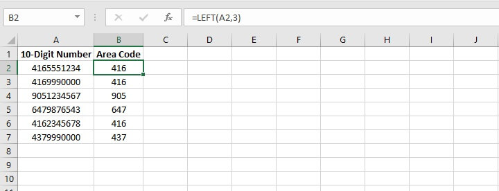

We already know that the area code will always consist of three digits, so this is the number entered in the num_chars argument. This type of scenario tends to be the most common application of the LEFT function.

Combining LEFT with LEN

What if your problem was a little more complicated? Maybe the values you want to extract are of variable lengths. For example, look at the scenario below.

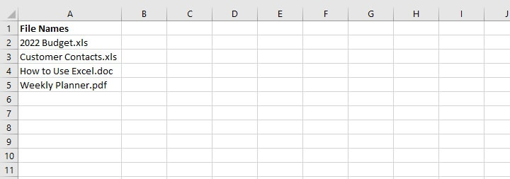
Here we have the names of four documents and their file extensions listed in Column A. We want to drop the extensions and extract just the file names. Of course, since the file names are of varying lengths, we can’t just enter a number in the num_chars argument and copy the formula.

The solution is to combine the LEFT function with LEN. The LEN function counts the number of characters within a text string. Since all the file extensions, plus the leading period are four characters in length, we can use this consistency to our advantage.

Our formula looks like this:

=LEFT(A2,LEN(A2)-4)

Let’s break down how this works, starting with the inner portion of the formula.

LEN(A2) counts the number of characters in the entire text string. The result would be 15. Excel stores this information in its memory. The result of 15-4 is 11. Therefore 11 now becomes the num_chars argument in our LEFT formula.

This is how we arrive at the formula:

=LEFT(A2,LEN(A2)-4)

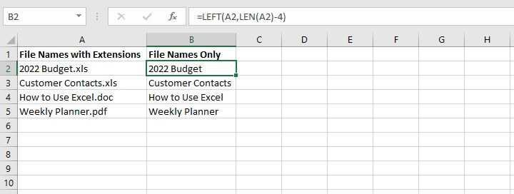Excel returns the first 11 characters from cell A2. Copying the formula to the other cells in Column B results in the same backend calculations which give us the file names only.

Since the LEN formula is set to calculate the number of characters before the file extension, it’s an excellent way to solve this particular problem.

Combining LEFT with SEARCH for strings of variable length

Let’s kick up the difficulty another notch. What if the file extensions didn’t all have the same number of characters?

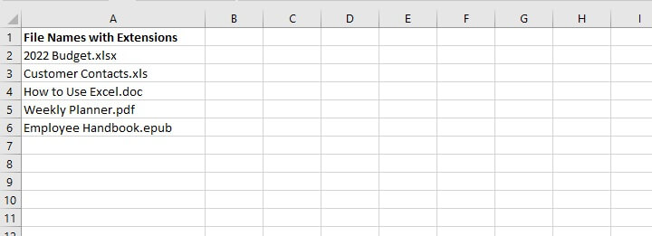We can’t use the number of characters after the period to come up with the value for the num_chars argument, but there is something they all have in common. All the file extensions are preceded by a period. So let’s use the period to our advantage!

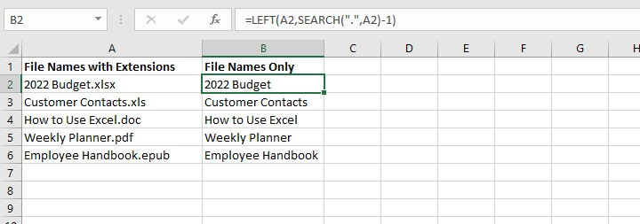
We can use the SEARCH function to locate the position number of the period and use the LEFT function to return all the characters to the left of the period.

=LEFT(A2,SEARCH(“.”,A2)-1)

SEARCH(“.”,A2) looks for a period within the A2 text string. The period is the 12th character. Since we want all the characters before the period to be returned by the LEFT function, we subtract 1.

If we plug this into the LEFT formula, it would read as follows:

=LEFT(A2,SEARCH(“.”,A2)-1)

Excel returns the first 11 characters from cell A2. When we copy this to the rows below, we get the names of all the files without their extensions.

Combining LEFT and SEARCH is also a great way to grab first names only from a “FirstName LastName” structure. Simply search for the space character. If there is only one space character, or if the first name appears immediately before the first space character, then you’re all set!

Combining LEFT with FIND for case-sensitive data extraction

Combining LEFT with FIND works in pretty much the same way as the LEFT/SEARCH combo, the only difference being that FIND is a case-sensitive search. This is illustrated below.

To extract 

=LEFT(A2,FIND(“Excel”,A2)-1)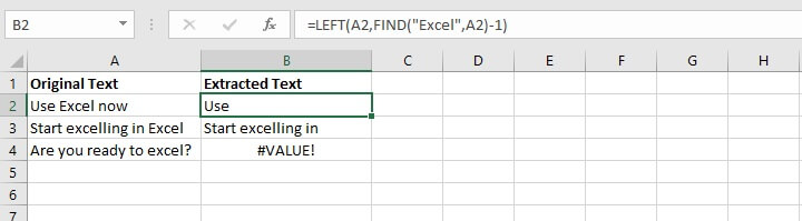

Notice that the formula in cell B4 returned a #VALUE! error, because there was no instance of “Excel” in a case-sensitive search of cell A4 using the FIND function.

Using LEFT, MID, and RIGHT functions to split data

LEFT is sometimes used with the MID and RIGHT functions. As their names suggest, MID is used to extract characters from somewhere in the middle of a text string, and RIGHT is used to grab the rightmost values from the string.

We usually use two or all of these functions when we want to break up a text string into separate pieces.

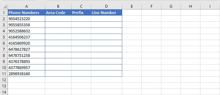
For example, the following dataset contains telephone numbers which we would like to split into three separate columns as follows:

• The area code, consisting of the first three numbers. 
• The prefix, consisting of the next three numbers. 
• The line number, consisting of the final four numbers.

Step 1

We would use the LEFT function to grab the first three numbers.

=LEFT(A2,3)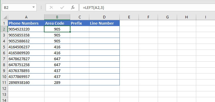

Step 2

Then we can use the MID function to get the next three numbers. The syntax of the MID function is:

=MID(text, start_num, num_chars)

• Text is the text string to be split.
• Start_num is the position number of the first character to be returned, counting from the leftmost character in text.
• Num_chars is the number of characters in text to return, starting with the leftmost character. 

All three arguments in the MID function are required.

=MID(A2,4,3)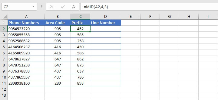

In the above formula, we ask Excel to extract three characters from the string in cell A2, starting with the fourth character from the left.

Step 3

Finally, we use the RIGHT function to extract the last four numbers. The syntax of the RIGHT function is:

=RIGHT(text, [num_chars])

• Text is the text string to be split.
• Num_chars is the number of characters in text to return, starting with the rightmost character. If omitted, only the rightmost character is returned.

=RIGHT(A2,4)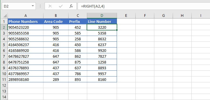

With the above formula, Excel extracts the four rightmost characters from the string in cell A2.

Now we have successfully split the text in one cell into three cells using a formula.

Excel LEFT function troubleshooting

There are a few times when you might not get the result you expected when using the LEFT function. Here are some common problems.

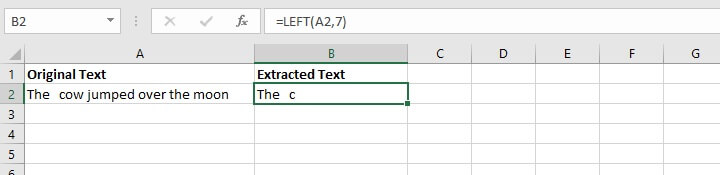
1. My LEFT formula returns fewer characters than I expected

If you know how many characters make up your desired output, but your LEFT formula only returns some of the characters, maybe there are extra spaces in your original text. 

Instead of removing them manually, you can simply use the TRIM function to remove them.

=LEFT(TRIM(A2),7)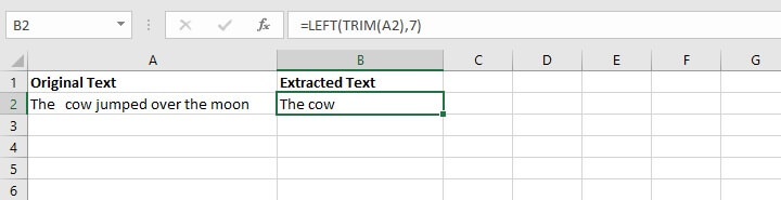

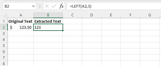
2. My currency symbol got dropped

If your original text had the Currency or Accounting format applied, the symbol is not a part of the characters in the cell. The symbol only appears because this is the display that comes with that particular number format. The LEFT function is a text function. Therefore, it will convert all values to Text format.

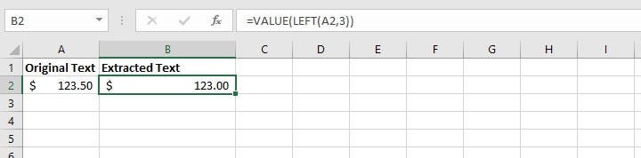
A useful workaround is to combine LEFT with the VALUE function to convert the text back to a number. Then you can select the number format you want. 

3. LEFT returns a weird value for my date

Remember, LEFT is a text function. It doesn’t handle numerical values well on its own. In the example below, we want to extract the day of the month from the dates in Column A.

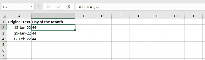In this case, LEFT just isn’t the best tool for the job. Dates are really just numbers displayed in a way that makes sense to us. But for Excel, the date displayed as “15-Jan-22” is stored as a number string (44576, to be exact).

So when we ask Excel to use the LEFT function to return the first two characters from that string, Excel says, “OK” and returns 44 — the first two numbers in the number string displayed as “15-Jan-22”.

The DAY function works better here.

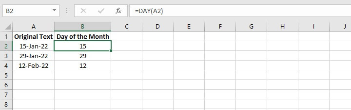And it’s easier too.

LEFT vs. LEFTB 

If you’re interested in learning about LEFTB, you’ll want to know that the only difference between LEFT and LEFTB is that LEFT returns the number of characters in a text string. LEFTB returns the number of bytes used to represent the characters in a text string.

LEFTB counts 2 bytes per character only when a double-byte character set (DBCS) language is set as the default language. The languages that support DBCS include Japanese, Chinese (Simplified), Chinese (Traditional), and Korean.

Otherwise, LEFTB behaves the same as LEFT, counting 1 byte per character. For this reason, we have only discussed LEFT in this resource.

Best tip for using Excel’s LEFT function 

Uses of the LEFT function aren’t limited to what we’ve discussed here. I’m sure you’ll think of other ways this little function can come in handy. 

The main thing to remember is to look for any element of consistency in your original dataset and use that to your advantage when trying to pull out pieces of text from a text string.

Learn more about Excel and other useful Excel functions by trying our Basic and Advanced course.

Ready to become a certified Excel ninja?

Start learning for free with GoSkills courses

Start free trial