Excel Custom Number Format - A Beginner’s Guide

---

Since you want to learn how to create an Excel custom number format, it seems fair to assume that you already know how to find and locate the built-in number formats provided by Excel. 

But we’d rather not take that for granted. Let’s cover the basics quickly, then dive into the nitty-gritty.

What is a number format?

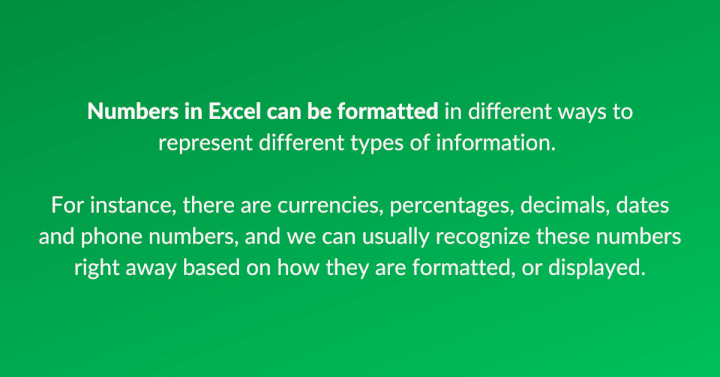
A number format controls how cells with numeric data appear in Excel. Numeric data can mean dates, time, money, or anything else that looks like a number. 

The most important thing to understand about number formats is that they only affect how the number looks — they don't change the actual value of the number that Excel uses in calculations.

You can find a list of built-in formats on the Home tab of the Excel ribbon in the Number command group. A dropdown field in that group displays the format of the active cell and allows you to change the number format of the active cell or highlighted cells by selecting another format from the dropdown list. 

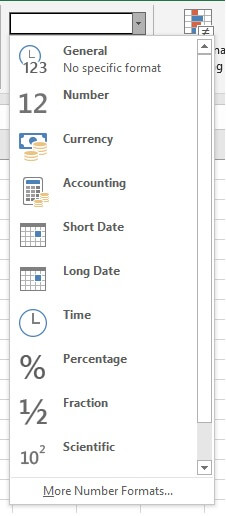The ‘Text’ number format is available by scrolling down and is used when you want to treat numbers as text.

Number format shortcuts

As an alternative to selecting from the dropdown list, you can also use the following keyboard shortcuts to apply number format changes to selected cells. These shortcuts work using the numbers above the letters on a Windows or Mac keyboard.

Excel defaults to the ‘General’ format unless it thinks that it recognizes the type of number you’re entering as currency, date, time, or something else.

Justification for additional number formats

With so many number formats available, why do we need to go adding to them by customizing number formats? 

Well, if you take a minute to think about it, it’s easy to see how even within each category above, there are multiple date, currency, and even percentage formats. For example, a date may be written as 09-Jan-2023, 1/9/23, or even Monday, January 9, 2023. Currency may be dollars ($), euros (€), yen (¥), and so on.

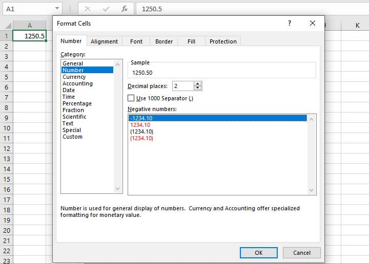
In the example below, the value 1250.5 was entered in cell A1. If we open the Format Cells dialog box using Ctrl+1 and select the Number category, we can see that we can increase or decrease the number of decimal places that will be displayed in this cell.

We can also use a checkbox to control whether a comma is displayed for values greater than or equal to 1000.

Further below, we can select the format for negative values (a leading dash, red font, parentheses, or red font in parentheses).

In some situations, there may be other types of number formats that are specific or unique to a given data set. Examples of this may include telephone numbers, account numbers, government ID numbers, etc. 

It makes sense that numbers of the same type should look consistent, and therefore may require a format not created by Excel programmers. I’m sure you can think of more examples like these.

This is why custom number formats are so useful, and in some cases necessary, for accurate representation of various types of numeric data.

Number format codes

Before we can go about building our own number formats, we need to be able to speak to Excel in a way that it understands.

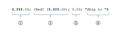
Number formats in Excel carry four sections of code. These sections are used to determine the formats for: 

• positive numbers 
• negative numbers
• zero values, and 
• text

in that order, and are separated by semicolons. 

Skipping sections in format code

Not all sections are required. When only one format is provided, Excel will use that format for all values.

If you create a format with two sections, the first section is used for positive values and zeros, and the second section for negative values.

To skip the first, second, or third sections, enter the semicolon where that section would be without entering a format. Those values will be hidden from the display.

To keep the default for any section, type General in that section, then enter the code for the section you want to change. For example, to keep the default display for positive and negative numbers, and display a dash for zero values, enter:

General; -General; "-"

Codes for formatting numeric data

The table below shows symbols that are used to control the appearance of strictly numeric data.

How to create a custom number format

Create a custom number format by doing the following:

1. Highlight the cell or range of cells that you would like to format.
2. Go to the Format Cells dialog box by clicking the Dialog box launcher, or Ctrl+1.
3. Select Custom from the Category pane on the left.
4. Use the scrollbar below the Type field to browse through the existing formats.
5. Single-click on one which has characteristics similar to the custom format you would like to create.
6. Go to the Type field and enter the codes you would like for your new format.

Note that this does not change the format which you selected. It creates a new custom format that is added to that worksheet for future use.

Still unsure of how to apply those codes to create a custom number format? Let’s do a simple example together, step by step.

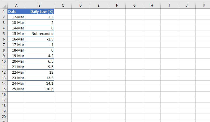
Scenario

In the worksheet shown below, we’ve recorded the daily low in Celsius. The Date format was automatically applied to Column A by Excel, and the default General format was applied to Column B. 

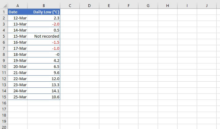
We want to apply the following format to Column B: 

• Positive values should be rounded to one decimal place. 
• Negative values should be displayed in red font, lead with a minus sign, and should be rounded to one decimal place. 
• Zero values should display a single digit - 0.

• Highlight the entire column by clicking on the Column B heading.
• Press Ctrl 1 on your Windows keyboard, or Command 1 on Mac.
• Select Custom from the Category pane.
• Single-click on an existing format to start your customization.

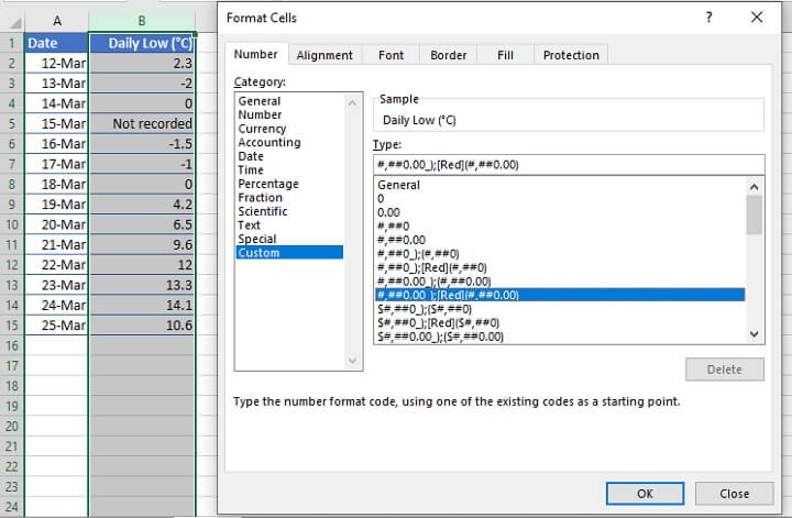
• Go to the Type field and enter: 0.0; [Red]-0.0; 0

removing all the extra characters.

For the example above, we’ve entered spaces after the semicolons for readability, but they are optional. 

• Click OK.

The Column B display is updated.

Other formatting codes

The following symbols may be used to format numbers as well as text.

Custom date and time formatting

To control the way dates and times appear, use the following codes.

It’s important to note the following:

• The above characters are not case-sensitive. For example, the code “M” is interpreted in the same way as “m”.
• The m or mm code must appear immediately after the h or hh code or immediately before the ss code. Otherwise, Excel displays the month instead of minutes.

Display literal character

The symbols we’ve used so far are meant to tell Excel how to treat the values we input into the cell. But there are times when we want those literal characters to be displayed as a part of the format. 

For instance, if we want the hash symbol (#) or question mark displayed, we would need a special way to indicate that. There is.

We use a backslash as an escape character to display the character which follows.

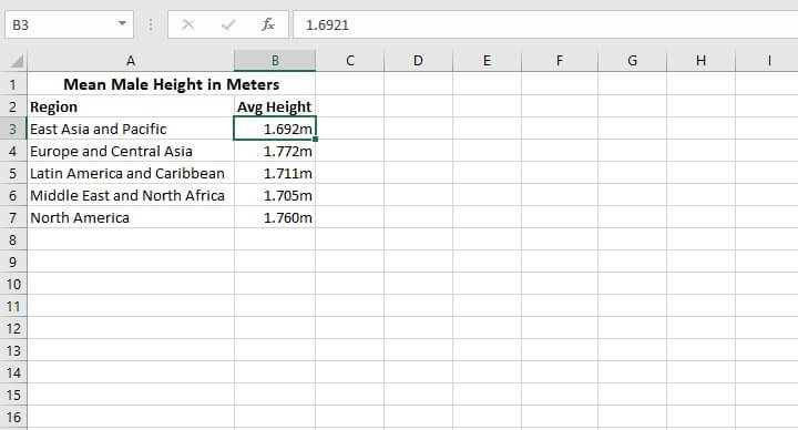
In the following example, we want to create a code where numeric values are rounded to three decimal places and are followed by the letter m (for meters).

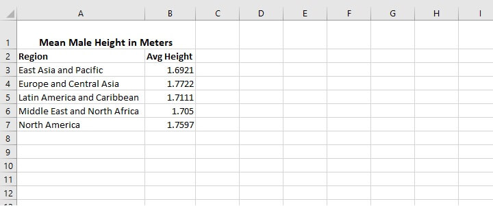Since we don’t want Excel to interpret “m” in the code as “month” or “minutes” we precede the code with a backslash.

0.000\m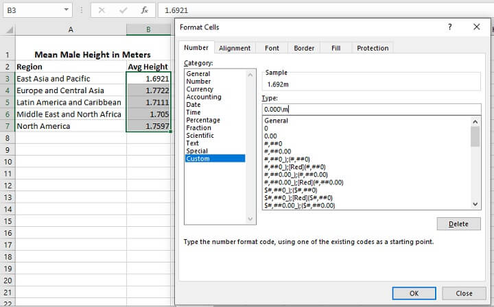

The display is updated to show the letter m after the selected values, even though the number entered has not changed.

When the following characters are used in the format code, they will be displayed as entered without the use of a backslash or double quotation marks.

How to edit or delete a custom number format

Existing number formats (whether built-in or custom) cannot be “edited” in the usual sense of the word. If you make a change to an existing number format, a new one is created which will appear in the Custom Category list for that workbook.

You can delete a custom format you no longer need by single-clicking on the format, then pressing the Delete button. If the Delete button is grayed out, that means the format selected is a built-in format and cannot be deleted.

Once you delete a number format, you cannot ‘undo’ that command. The format has to be re-created.

Color formatting

You can change the default black font color to any of the following eight colors by enclosing them in square brackets in the respective code section.

• [Black]
• [Blue]
• [Cyan]
• [Green]
• [Magenta]
• [Red]
• [White]
• [Yellow]

Display text without converting cell to text format

If you type text along with numeric values in a cell, Excel automatically converts that cell to a text format, making it unusable for formulas and other mathematical calculations. If you want a specific text displayed next to a number without changing the number to a text format, you may want to consider adding the text value to the number code.

For example, to add the text “Profit margin is ” you would use the following code:

“Profit margin is ”General%

If this is the only code entered, any negative values entered would have a minus sign before the text display. To avoid this, you may want to add the negative code section. Your custom format would look something like this:

"Profit margin is "0.0%;[Red]"Profit margin is "-0.0%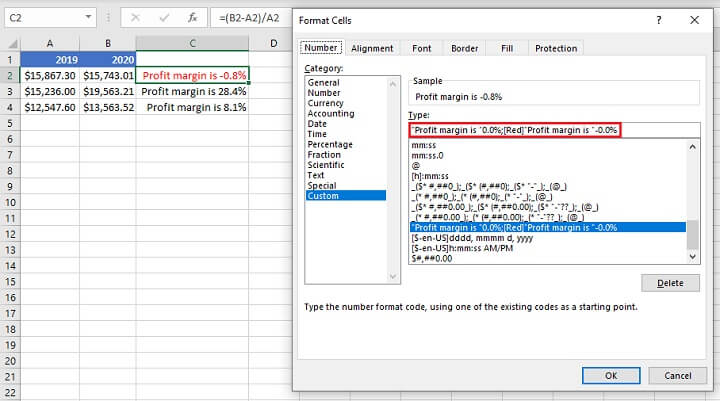

Conclusion

You won’t be able to learn all the possible code combinations in this short read, but you’re probably a lot more knowledgeable about how Excel custom number formats work now. Hopefully, this will help you get around some of those pesky display problems you’ve been having.

Learn more about how you can become an Excel ninja with GoSkills Excel courses. We recommend the Excel - Basic and Advanced course.

Level up your Excel skills

Become a certified Excel ninja with GoSkills bite-sized courses

Start free trial