How to Use the Excel SEARCH Function

---

The Excel SEARCH function does exactly what it sounds like. It searches for a character or group of characters within a text string and lets you know where that substring is by returning the position number of the first character you searched for.

Syntax

The syntax of the Excel SEARCH function is as follows:

=SEARCH(find_text,within_text,[start_num])

• Find_text - is the substring or character you want to locate.
• Within_text - is the text string or cell reference within which you will look for your character(s).
• Start_num - (optional) is the position number of the character where you want your search to start. If the third argument is omitted, SEARCH starts looking from the first character of the string.

Good to know

• Arguments stated as explicit text must be placed within double quotation marks.
• Arguments stated as cell references should not be placed within double quotes.
• The SEARCH function is not case-sensitive. If you want to perform a case-sensitive search, the FIND function is a better choice.
• If no match is found, SEARCH returns a #VALUE! error.
• The SEARCH function supports the use of wildcards.

---

---

Basic application

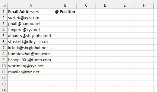
In the following list of email addresses, we might want to know the position number of the “@” symbol.

In this example, there is no need to specify the third argument (start_num) since we only anticipate one @ symbol in each email address.

=SEARCH(“@”,A2)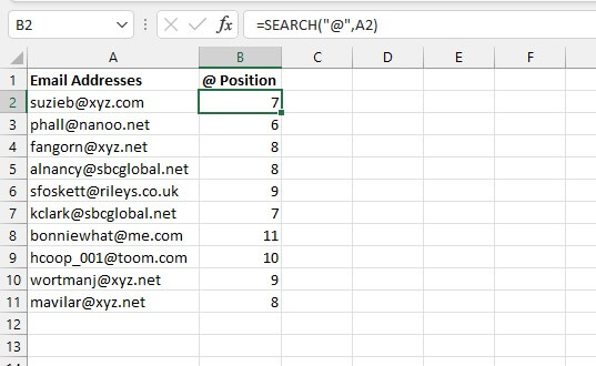

There are several ways in which this function can be incredibly useful.

Test for the presence of a text string

SEARCH can be combined with ISNUMBER to test for the presence of a substring. ISNUMBER simply tests whether the value being evaluated is a number or not, the logic being that if a position number is returned by SEARCH, the ISNUMBER formula will return a value of TRUE. And if SEARCH returns a #VALUE! error, ISNUMBER will return a value of FALSE.

The ISNUMBER function syntax is:

=ISNUMBER(value)

So we can simply make our SEARCH formula the argument of the ISNUMBER formula.

=ISNUMBER(SEARCH(“xyz.net”,A4))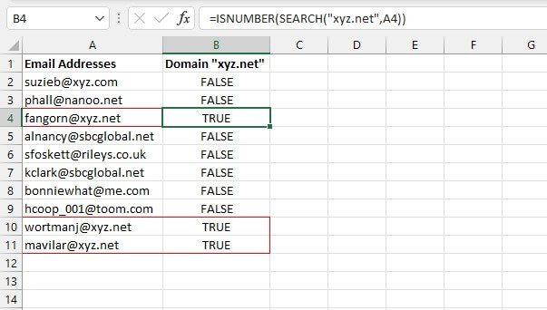

The above formula identifies whether a text string contains the substring “xyz.net.” If it does not contain that substring, the formula returns a value of FALSE.

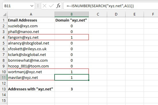
Alternatively, we can place two minus signs before the ISNUMBER function, which will cause the formula to return 1 or 0 for TRUE or FALSE, respectively. It then becomes a simple thing to add the number of addresses that have a “xyz.net” domain by using the SUM function.

This principle can be extended to accommodate a customized response using the IF function. 

The IF function evaluates a logical statement and returns a customized response if the statement evaluates to TRUE and a different customized response if the statement evaluates to FALSE. 

With this principle, we can tell Excel what to do if ISNUMBER returns a TRUE response and what to do if it does not.

The syntax of the IF function is:

=IF(logical_test, [value_if_true], [value_if_false])

So we can simply make our ISNUMBER/SEARCH formula combination the first argument of the IF formula.

=IF(ISNUMBER(SEARCH(2,A2,5)),"Yes","No")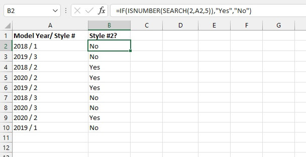

Note that in the above example, we used all three arguments of the SEARCH function. This allowed us to search for the value “2” starting with the 5th value. 

The optional start_num argument is usually used in situations where the substring being searched for appears more than once, and we would like to ignore a certain number of initial occurrences. By specifying the start number, we get SEARCH to ignore the digits in the year. 

Beginning with the 5th character, if the number “2” is found, the SEARCH function returns the position number, resulting in a TRUE output by the ISNUMBER function. The IF function is then written to return the text “Yes” for TRUE results and “No” for FALSE results.

Note: Searching for a numeric value works with or without the double quotation marks.

Replace a substring if present

SEARCH can be combined with the REPLACE function to replace one substring with another if it is present in the original text string. The syntax of the REPLACE function is:

=REPLACE(old_text, start_num, num_chars,new_text)

The meanings of these arguments are as follows:

• Old_text - is the text string containing the substring to be replaced.
• Start_num - is the starting position number of the text to be replaced.
• Num_chars - is the length of the text to be replaced. 
• New_text - is the text that will replace the characters you want to remove.

Below, we might want to search for the word “song” and replace it with the word “poem” if it is present.

=REPLACE(A2,SEARCH("song",A2),4,"poem")

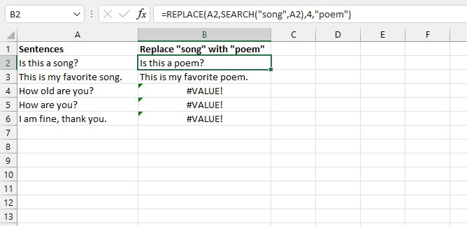The result of the SEARCH formula was used as the start_num argument of the REPLACE function since a position number is needed, and the exact location of the “song” substring within the text string is unknown. 

With this formula, cells that do not contain the text searched for return a #VALUE! error. This can be avoided by incorporating the IFERROR function to return an alternative result.

The syntax of the IFERROR function is:

=IFERROR(value, value_if_error)

By using the REPLACE/SEARCH formula combination as the value argument of the IFERROR function, we can alter cells that contain the values we searched for without changing the others.

=IFERROR(REPLACE(A2,SEARCH("song",A2),4,"poem"),A2)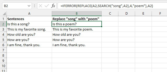

The last argument of the IFERROR function above is set to return the original text in column A if no match is found by the SEARCH argument.

Extract a substring from a larger text string

The SEARCH can be combined with the LEFT, RIGHT, and MID functions to extract characters from a text string by locating a character or the beginning of a text string and then using that information to extract the desired substring.

Extract leftmost characters

We can extract the usernames from the email addresses by using the SEARCH function as an argument of the LEFT function.

The LEFT function extracts the specified number of characters from a text string, beginning with the leftmost character, with an optional argument being the number of characters to return. The syntax of the LEFT function is:

=LEFT(text, [num_chars])

Since the SEARCH function returns the position number of a character or text string, this position number can be used as the num_chars argument of the LEFT function. We typically subtract 1 from that position number to get the “stop” position of the string we want to extract.

=LEFT(A2,SEARCH(“@”,A2)-1)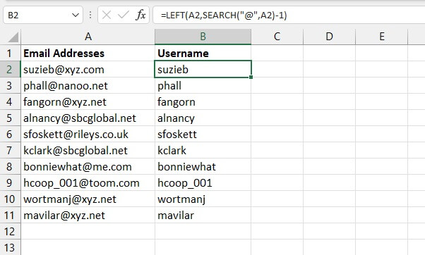

By locating the position number of the @ symbol, we can determine that the username ended with the previous character, meaning we need to subtract 1 from the result of the SEARCH formula. This becomes the num_chars argument of the LEFT formula.

Extract rightmost characters

If, on the other hand, we wanted to extract the domain name from the text string, we could do this using either the RIGHT and LEN functions together or, with a little creativity, the MID function. Both options are shown below.

Option 1

The LEN function counts the number of characters in a text string with the following syntax:

=LEN(text)

The RIGHT function returns the specified number of characters from a text string counting from the rightmost character. The syntax of the RIGHT function is:

=RIGHT(text, [num_chars])

We will now use the LEN/SEARCH formula combination as the num_chars argument of the RIGHT formula.

=RIGHT(A2,LEN(A2)-SEARCH("@",A2))

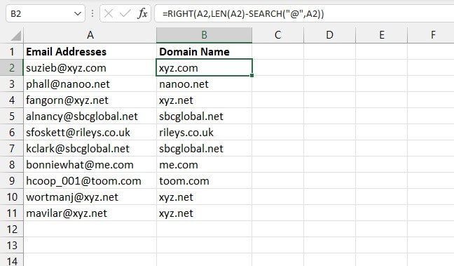Once SEARCH determines the position number of the @ symbol and we subtract that position number from the length of the text string (courtesy of LEN), we are left with the number of characters that make up the domain name. This then becomes the num_chars argument of the RIGHT function.

Option 2

Our second option is even simpler. We can use the MID function to grab characters that begin in the middle of a text string and go all the way to the end. The syntax of the MID function is:

=MID(text, start_num, num_chars)

Though all the arguments are required, it is useful to know that MID allows us to treat the entire string after the dash as a middle string by specifying a number that is very large. For the sake of this example, we can use 100. 

=MID(A2,SEARCH(“@”,A2)+1,100)

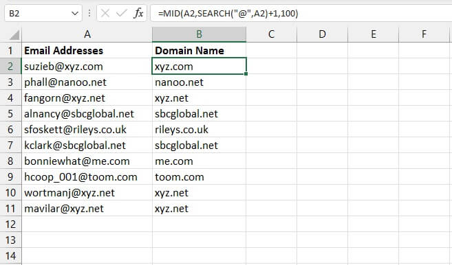We have used SEARCH to determine the position of the “@” character. Adding 1 to that position number tells us the starting position (or start_num) of the MID function.

Extracting characters from the middle of a text string

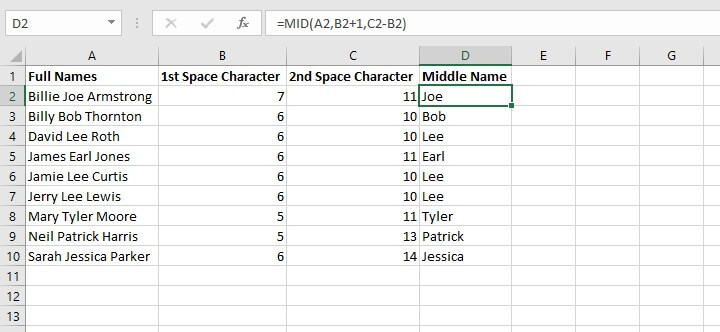
How about trying to extract text of variable length that is actually in the middle of a text string, like getting the middle names from the following list? 

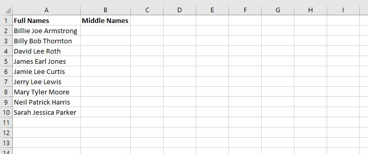Since the names are all of different lengths, we need to use some combination of the MID and SEARCH functions to isolate the two space characters and grab the text in-between. 

Step 1

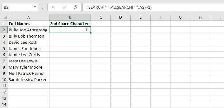
The first step is simple. We need to find the position number of the first space character. We can use the standard SEARCH formula without the optional argument.

=SEARCH(“ ”,A2)

The result is 7. This means the first space character is in the seventh position of the text string. So by adding 1 we know that the middle name starts with character number 8. 

=SEARCH(“ ”,A2)+1

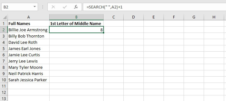This information will later be used as the start_num argument of the MID function.

But now, how do we know where the middle name ends? That is, what will we use to determine the num_chars? We need to identify the position of the second space character in the original text, which requires a little bit of Excel function gymnastics.  

We can think about it this way. Assuming that we start looking from the 8th character in the string, where would the next space character be?

Step 2

We already know that SEARCH(“ ”,A2)+1 tells Excel where the middle name starts, so let’s use that same location to start searching for the next space character.

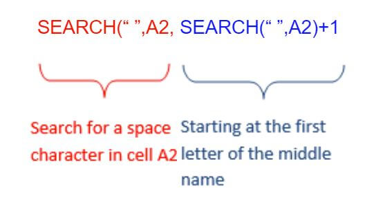This formula will return the position number of the second space character from the original text string.

Step 3

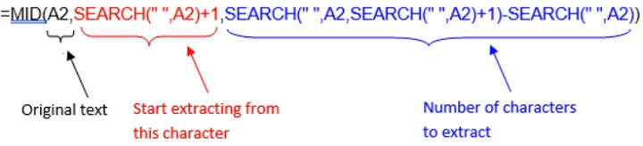
The only thing left to do now is to use the MID function to look at the text in cell A2 (text argument), and starting with the eighth character (start_num argument), extract three characters (num_chars argument).

SEARCH(" ",A2,SEARCH(" ",A2)+1)-SEARCH(" ",A2))

The final SEARCH(“ ”,A2) element ensures that the number 11 will be subtracted from the position number of the first space character. 

We now pull all these elements together as arguments of the MID function.

 

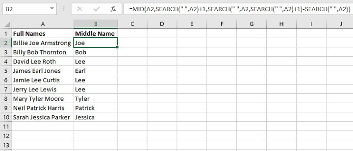This formula gets the job done, but you might not be quite comfortable working with so many nested functions just yet. If that’s true, then you might find it easier to create helper columns for rough work and use the result of those formulas to get the same results.

After Step 1 above, just determine the location of each space character step by step, and use those cell references as the arguments for the MID function.

Using wildcards to search

Wildcards are useful when the exact substring is unknown, or when a partial match is accepted.

The SEARCH function supports the use of the following wildcards: 

In the following example, we are searching for the substring “cent” regardless of whether it appears at the beginning, middle, or end of a text string.

=SEARCH(“cent*”,A2)

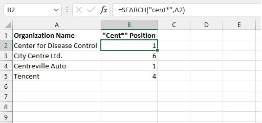The SEARCH function returns the position number of the first character in the substring. As pointed out at the outset, it does not matter whether the text is uppercase or lowercase.

If we wanted to search for “center” or “centre” we could accommodate both spellings by making use of the ? wildcard instead.

=SEARCH(“cent?? ”,A2)

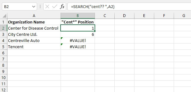With this search, only strings with the letters “cent” followed by exactly two characters and a space are considered matches. Text strings that do not fit this criterion return a #VALUE! error.

In the following example, we want to find out the number of characters in sentences that ask a question. 

=SEARCH(“~?”,A2)

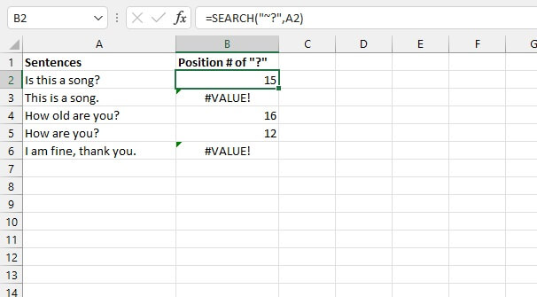Since the question mark is a wildcard, we will run into problems if we simply search for “?”. The tilde acts as a sort of “escape” character so that characters that are generally used as wildcards can be interpreted literally by Excel.

SEARCH vs. SEARCHB 

If you’re interested in learning about the SEARCHB function, you’ll want to know that the only difference between SEARCH and SEARCHB is that SEARCHB counts 2 bytes per character when a double-byte character set (DBCS) language is set as the default language. The languages that support DBCS include Japanese, Chinese (Simplified), Chinese (Traditional), and Korean.

Otherwise, SEARCHB behaves the same as SEARCH, counting 1 byte for each character. For this reason, we have only discussed SEARCH in this resource.

Other ways to find things in Excel

The Excel SEARCH function is meant to help you look for something within a specific text string. But if you want to lookup an item within an Excel table or data set, the VLOOKUP or HLOOKUP function might be more suited to do the trick. If you have Excel 365, XLOOKUP is even more flexible, as it can do everything the previous functions can do and more. 

On the other hand, if you’re looking for non-formula methods to locate text in Excel, you might want to check out this resource to learn how to find and replace one text string with another text string.

Explore our Excel course library for other cool Excel tips. You can start with the Excel - Basic and Advanced course.

Ready to become a certified Excel ninja?

Start learning for free with GoSkills courses

Start free trial