XLOOKUP in Excel: A Beginner's Guide

What is XLOOKUP in Excel?

The XLOOKUP function in Excel is being hailed as the replacement for both VLOOKUP and HLOOKUP, hence the “X” standing in for either character.

Like its predecessors, XLOOKUP looks for a value in a table and returns a matching result.

But whereas the other lookup functions require complex pairing with other functions like INDEX/MATCH to search in different areas, or IFERROR to display a customized message, XLOOKUP comes with those functionalities built in.

And who wants to type two formulas instead of just one?

A huge game-changer is that VLOOKUP and HLOOKUP formulas assume that you’ll accept near-matches, and that your data is already sorted. By contrast, no sorting is necessary with XLOOKUP, and searches default to an exact match. 

For now, XLOOKUP is only available in Excel 365, so if you’re using an older version you won’t be able to try out this shiny new functionality. But a nice alternative is that it is available in the browser-based Excel with Office online.

---

---

Overall, XLOOKUP in Excel is far more versatile. By looking at the syntax, we can see a few arguments which aren’t used in VLOOKUP or HLOOKUP. Let’s break them down.

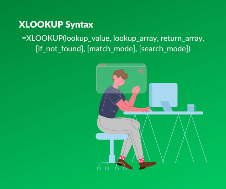
Syntax

Argument definitions

1. Lookup_value – the value you want to search for        
2. Lookup_array – the list where you want Excel to search for this value
3. Return_array – the list from which you want the result
4. If_not_found – what to display if the lookup value doesn’t exist (optional)
5. Match_mode – exact match only, or accept approximate matches (optional)
6. Search_mode – search first to last, or reverse order (optional)

Argument 1: Lookup value

=XLOOKUP(lookup_value, lookup_array, return_array, [if_not_found], [match_mode], [search_mode])

Lookup_value is the value that you want Excel to search for. There is no change here.

Argument 2: Lookup array

=XLOOKUP(lookup_value, lookup_array, return_array, [if_not_found], [match_mode], [search_mode])

Lookup_array is where you want Excel to look for the lookup value. This is comparable to the first column in VLOOKUP’s table_array, or the first row in HLOOKUP’s table_array. The main difference here is that we don’t reference an entire table at this point, just the range that may contain the value we want to search for.

Argument 3: Return array

=XLOOKUP(lookup_value, lookup_array, return_array, [if_not_found], [match_mode], [search_mode])

Return_array is the array or range containing the values you want Excel to show as the result. An important point to note is that the length of the lookup and return arrays must be the same.

For example, if your search column is 16 rows long, your return (result) column should also be 16 rows long so that there is always a row to match the value that was found. If not, you’ll get a #VALUE error.

Argument 4: If not found

=XLOOKUP(lookup_value, lookup_array, return_array, [if_not_found], [match_mode], [search_mode])

A useful feature with XLOOKUP is that it allows you to tell users, in everyday language, that the value they are searching for doesn’t exist in the lookup array. For example: 

=XLOOKUP(B12,A3:A10,G3:G10,“This value doesn’t exist”,0)

If the user types a value in cell B12 that is not found in the A3:A10 range, they will see the response “This value doesn’t exist.” Remember to put your text in double quotes (“ ”). This argument is optional, but it’s far better for an end-user to see “This value doesn’t exist.” If nothing is entered in Argument 4, you will see an “#NA” error. 

Argument 5: Match mode 

=XLOOKUP(lookup_value, lookup_array, return_array, [if_not_found], [match_mode], [search_mode])

XLOOKUP searches for an exact match by default. This means that if we want Excel to search only for what was entered in the lookup_value cell, we can either type 0 in Argument 5, or simply leave it blank, since that’s the default. If no exact match is found, Excel will return a #NA error, or whatever was entered in Argument 4. 

But if you do want to accept approximate matches, Argument 5 allows you to do that. The possible options for Argument 5 are:

0 exact match only (default)

-1 exact match or closest value smaller than lookup value (approximate smaller)

1 exact match or closest value larger than lookup value (approximate larger)

2 wildcard match.

Approximate smaller match

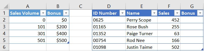
Let’s say you’re giving a staff incentive based on sales volume as shown below. The numbers in the “Sales Volume” column are the lower limits to qualify for the amounts in the “Bonus” column. So employees who made 0-100 sales wouldn’t qualify for the incentive, but employees who made 301-500 sales would get $400.

Next to that is another table which has the names of the employees and their individual sales performance.

To get Excel to determine the bonus amount for each employee in column H, XLOOKUP offers a simple solution.

Using our XLOOKUP function syntax, we know that our lookup_values will be found in column F, our lookup_array in column A, our return_array in column B, and we will accept approximate matches since employees’ sales figures may not be exactly what’s in column A.

Our formula looks like this:

=XLOOKUP(F2,A2:A5,B2:B5,,-1)

This will ensure that employees like Rod Nee will receive $200 for his 166 sales, but Paige Turner will not receive a bonus as she only made 63 sales.

Approximate larger match

At other times, we want Excel to find the closest value larger than the lookup value if an exact match is not found. In these instances, we type 1 in Argument 5. For example:

=XLOOKUP(D2,A2:A5,B2:B5,,1)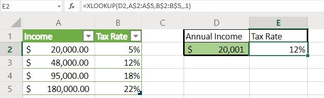

In the example above, table A1:B5 states the rate at which income taxes are applied. An amount higher than the stated amount will fall in the higher tax bracket. In this case, the employee made just $1 over $20,000. Because we entered 1 in Argument 5, Excel correctly applies the higher tax rate of 12%. 

Wildcard match

Sometimes we want Excel to perform a partial or “fuzzy” match, such as in the case of alternative spellings of a name. In this instance, we type 2 in Argument 5 of the XLOOKUP function. 

For example:

=XLOOKUP(B12,B2:B8,D2:D8,"Name not found",2)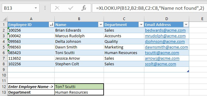

In the example above, we want to know which department an employee works in. The formula in cell B13 allows the user to enter a wildcard in cell B12 if they are uncertain of the way an employee’s name is spelled. 

If only a single character is unknown, we use a question mark in place of the unknown character. For example, to allow a search for “Tony Scutti” or “Toni Scutti”, the user would enter “Ton? Scutti” in cell B12.

An asterisk represents any string of characters, which would allow Excel to search for spellings of “Bryan”, “Brian”, or “Brien”, by typing “Br*n Edwards” in the input cell.

Argument 6: Search mode

=XLOOKUP(lookup_value, lookup_array, return_array, [if_not_found], [match_mode], [search_mode])

By default, XLOOKUP will start searching from the first item in the lookup array. There may be times that we want to start searching from the last value instead. Search behavior is controlled by Argument 6, search_mode, which is optional.

The possible options for search mode are:

1 first to last (default)

-1 last to first (reverse) 

2 binary search values sorted in ascending order 

-2 binary search values sorted in descending order 

Using XLOOKUP to return multiple values

It’s also possible to return multiple values using the XLOOKUP formula. The number of values you hope to return must match the number of empty cells available next to the input cell, that is, to return 3 values, you need 3 adjacent empty cells.

An example is shown below:

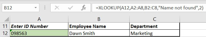
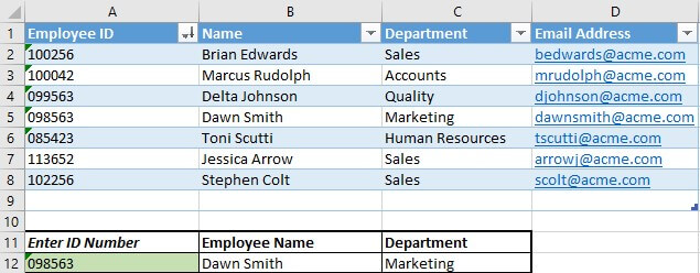In the above scenario, we want cells B12 and C12 to show the employee name and department for the ID number entered in cell A12. For that, simply include the entire range of possible results as our return array, in this case, cells B2 to C8. We enter the formula in cell B12 and there is no need to re-type the formula in cell C12, as the inclusion of the two adjacent columns (B and C) in our return array instructs Excel to “spill” the adjacent result into cell C12.

Selecting cell B12 will show the formula we entered in the formula bar as expected.

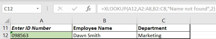
The formula will also appear if we select cell C12, but will be greyed-out and non-editable.

So now you know all about this powerful new function - XLOOKUP in Excel. It’s a timesaver, and will likely become the most popular function from the lookup family. 

Try out the above scenarios yourself by downloading the free practice file.

Learn more

Explore our Excel courses now to learn about this and the other awesome elements of Excel! 

Ready to become a certified Excel ninja?

Start learning for free with GoSkills courses

Start free trial