How to Use the SUM Function in Excel

---

One of the best functions for beginners to learn is the SUM function in Excel. It is a quick demonstration of how Excel functions can be used to simplify your otherwise manual calculations. 

Aside from being able to add cells and explicit values in Excel, the SUM function can also be combined with other functions to create powerful features and capabilities.

Let’s go over the basic Excel SUM formula, then look at some examples of how we can expand on it.

Free Excel crash course

Learn Excel essentials fast with this FREE course. Get your certificate today!

Start free course

Syntax

=SUM(number1,[number2],...)

Arguments in the SUM function may be an explicit number, cell reference, or cell range. SUM accepts a minimum of one argument and a maximum of 255. Arguments, including non-contiguous cell references, are separated by commas.

The return value is the sum, or total, of the numbers or referenced values within parentheses.

---

---

Why use a function?

The SUM function adds numbers. That’s neither surprising nor earth-shattering. But you may wonder why we need a special function to do that when the plus sign works just fine.

The first and most obvious reason is, of course, efficiency, especially in the case of a range of cells. It’s far quicker to type “SUM” and highlight the range to be added than it is to type each value one by one.

Here is another advantage of the SUM function. It’s true that you’ll get the same results whether you use the plus sign or SUM in the following example.

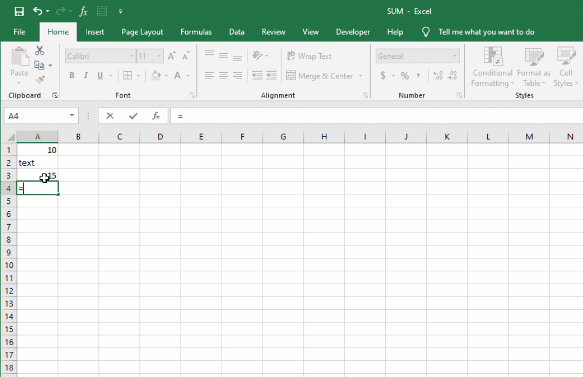
However, an error results if the plus sign is used when one cell includes a text value. The SUM function ignores text values, so a valid result is returned.

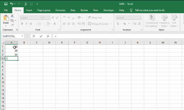
AutoSum

AutoSum is a quick way to sum a range of cells. It automatically enters a SUM formula in the selected cell.

To autosum:

1. In the row below the cells you want to sum, you can select the blank cell. 
2. From the Home tab on the Ribbon, click the AutoSum command (Σ symbol) or use the keyboard shortcut (Alt + =).
3. A SUM formula will appear in the active cell with a reference to the numeric cells immediately above.
4. Press Enter.

This method can be useful for adding an entire column or row of values without scrolling to the first cell in the range.

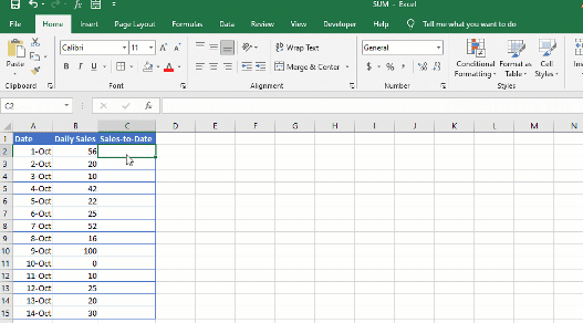
Calculate a running total

Sometimes we want a formula that progressively adds values up to the most recent value entered. This allows you to see what a total was up to a particular point in time (for example, month-to-date, year-to-date, etc.). This is called a cumulative sum.

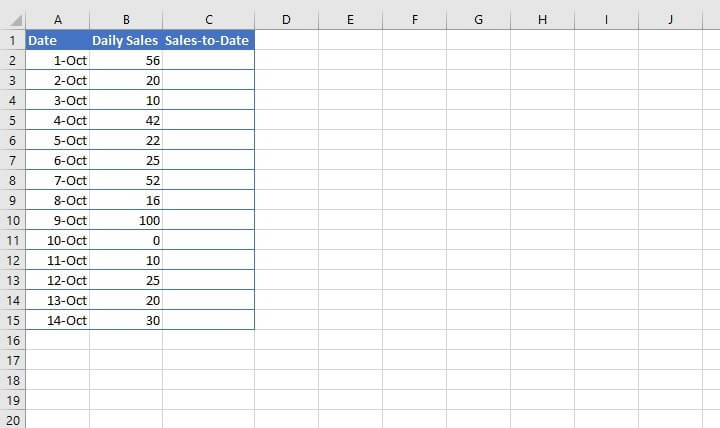The simplest way to achieve this is to create an expanding reference by making use of absolute (fixed) and relative cell references.

To do this, the first output cell will start and end with the same cell reference, as its range, B2:B2. The first reference to cell B2 should then be anchored with dollar signs to create a fixed reference, but the second instance remains relative. 

This setup ensures that when the formula is copied to the cells below, the range will always start at B2, but will expand to include up to the previous entry.

Note that it may be necessary to click ‘Ignore Error’ to remove the green Trace Error flag.

Sum range with errors

If a range contains cells with error values, the SUM function will also return an error. 

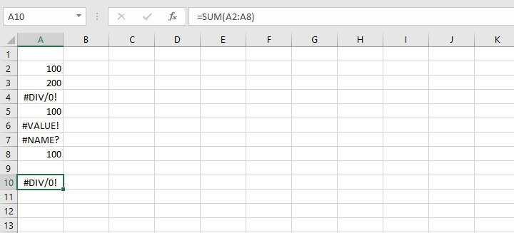The way to get past that is to pair the SUM and IFERROR functions into an array formula.

Remember that IFERROR is able to return an alternative value or calculation if a cell or formula results in an error. The syntax of the IFERROR function is:

=IFERROR(value, value_if_error)

• Value is the argument, calculation, or cell reference which is checked for an error.
• Value_if_error is a customized value or calculation to return if the first argument is evaluated to be an error. 

We will ask Excel to:

1. Substitute a value of zero wherever an error occurs with the IFERROR function. 
   • IFERROR(A2:A8,0)
2. Find the sum of the values within that range.
   • SUM(IFERROR(A2:A8,0)
3. Add all the values by pressing Control + Shift + Enter all at once.
   • {SUM(IFERROR(A2:A8,0)}

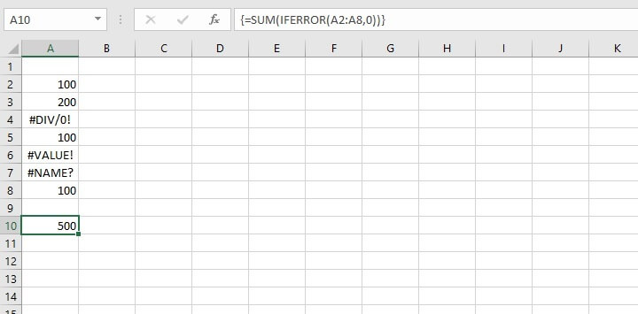Note that you should not type the curly brackets yourself. Pressing Control + Shift + Enter creates an array formula (sometimes called CSE formula), denoted by the automatically-inserted curly brackets. Excel interprets this array formula as an instruction to evaluate each cell within the range one by one, then find the sum of the values within the range.

The SUM formula above therefore sees SUM(100, 200, 0, 100, 0, 0, 100) and returns a result of 500.

SUM based on criteria

Sometimes there are special sum-type functions we’d like to perform — like only add cells that satisfy certain criteria. Or the reverse — exclude certain values from a total. Below are some of the types of problems that can be solved with modifications to the Excel SUM function.

Each function is a topic in its own right but is briefly explained here. For more detailed examples of how to use these functions, click on the respective link to jump to that resource.

SUMIF: Sum cells that match a single criterion

The SUMIF function combines the concept of “IF” (conditionality) with the “SUM” functionality. SUMIF adds numbers within a range that meet a single given condition. To do this, SUMIF needs the range it should be looking at and the criterion it should look for.

The syntax, or format, of the SUM function is:

=SUMIF(range,criteria, [sum_range])

• Range - the range of cells to be evaluated.
• Criteria - the condition (number, text, or expression) that each cell must satisfy.
• Sum_range - the actual cells to sum (optional). If omitted, the range will be used. 

The optional argument, sum_range, is the range to be used if the values to be added are not in the range to be searched. 

=SUMIF(B2:B10,“north”,C2:C10)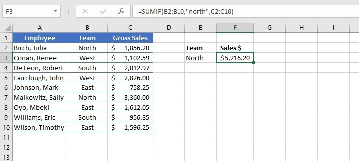

The above formula searches the range B2 to B10 for the text value north. The text criterion is placed in double quotes and is not case sensitive. When the value is found, Excel performs the SUM function on corresponding values in the range C2 to C10.

SUMIF also works with logical operators (<, >,=) when stating criteria, so: 

=SUMIF(C2:C10,">=1000")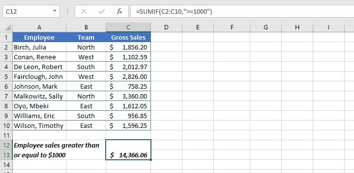

In the above example, the values to be added are in the range being searched, so no sum_range is necessary.

SUMIFS: Sum cells that satisfy multiple criteria

The SUMIFS function takes SUMIF a step further by adding cells that satisfy multiple user-defined criteria. A total of 127 pairs of criteria may be submitted in a single SUMIFS formula.

The SUMIFS syntax is:

=SUMIFS(sum_range, criteria_range1, criteria1,[criteria_range2], [criteria2]...)

• Sum_range - the range of cells to be added.
• Criteria_range1 - the range of cells to be evaluated.
• Criteria1 - the condition that cells in criteria_range1 must satisfy. 
• Criteria_range2 - the second range of cells to be evaluated.
• Criteria2 - the condition that cells in criteria_range2 must satisfy.

All arguments after criteria1 are optional.

In the example below, we can use SUMIFS to find the sum where employees on the East team made more than $1000 in sales.

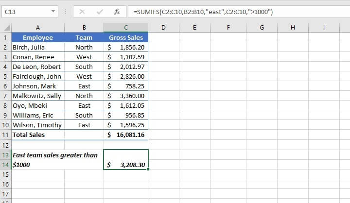Note that in the case above, all the conditions within the formula must be met to be included in the values being added. Even if one condition fails, that value is excluded from the total. In this sense, it uses a logic similar to the AND function.

SUMIF + SUMIF: Sum cells that satisfy at least one of multiple criteria

The SUMIF function identifies and adds cells that satisfy a single condition, while the SUMIFS function singles out and adds only those cells that satisfy all the stated conditions.

However, what if you want to state several conditions and find the sum of cells that satisfy any (at least one) of the stated conditions? This sounds like the way the OR function works. But there are two reasons the OR functionality cannot be combined with SUM to solve this problem:

1. OR can only evaluate a single cell at a time. It cannot evaluate a range of cells.
2. OR is a logical value, and returns TRUE or FALSE, which is not compatible with the adding of values.

So how do we accomplish this task? Sadly, there is no one function for finding the sum with multiple OR criteria, but we can make use of multiple SUMIF formulas to get around this limitation.

Let’s add the sales made by employees who were either on the North or the South teams.

=SUMIF(B2:B10,"North",C2:C10)+SUMIF(B2:B10,"South",C2:C10)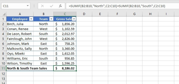

The first formula identifies cells in the range B2 to B10, which contain the word North and sums the corresponding figure in column B ($1,856.20 + $3,360).

The second formula identifies cells in the range B2 to B10, which contain the word South, and sums the corresponding figures in column B ($2,012.97 + $956.85).

The grand total of $8,186.02 is displayed in cell C11.

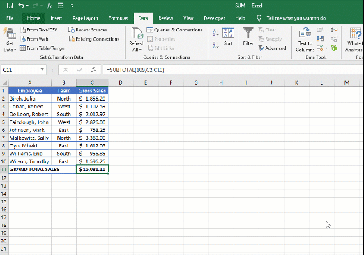
SUBTOTAL: Sum specific items in a filtered list

There is another less-known function that adds cells in Excel. SUBTOTAL can perform a number of tasks, including SUM, AVERAGE, COUNT, PRODUCT, among others. 

By default, SUBTOTAL excludes values in rows hidden by a filter, which gives SUBTOTAL a decided advantage over the SUM function in this regard.

The syntax of the SUBTOTAL function is:

=SUBTOTAL (function_num, ref1, [ref2], ...)

• Function_num - Excel-defined function number to be used.
• Ref1 - a named range or reference to subtotal.
• Ref2 - a named range or reference to subtotal (optional).

Functions within SUBTOTAL are numbered from 1-11 and presented as options while the formula is being entered. Those same functions are also presented in the 100-series to indicate that the SUBTOTAL should exclude any rows that are manually hidden.

For example, SUBTOTAL function 9 maps to the SUM function, adding all cells within the range, even those which have been manually hidden. Function 109 also maps to the SUM function but excludes those cells which are manually hidden.

Since SUBTOTAL is meant to work with data in columns, finding a subtotal of a horizontal range will add all values within that range, whether or not there are hidden values.

A key advantage of the SUBTOTAL function is that it always ignores values in cells that are hidden by an Excel filter. Values in rows that have been "filtered out" are never included, regardless of function_num.

Another point of note is that SUBTOTAL also automatically ignores other SUBTOTAL formulas that exist in references to prevent double-counting, as shown below.

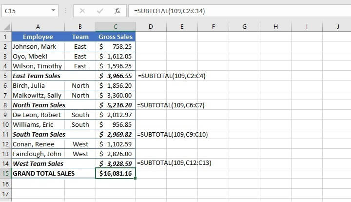The grand total shown in cell C15 represents the sum of all team sales without adding each team’s subtotal, which was calculated using the SUBTOTAL function.

Summary

So you’ve learned how to use the SUM function in Excel, and as a bonus, other functions within the SUM family. 

Just getting started in Excel? Try our free Excel in an Hour crash course to cover some basics in Excel.

Free Excel crash course

Learn Excel essentials fast with this FREE course. Get your certificate today!

Start free course