
With the SUMIF Excel function, we can quickly add numbers within a range that meet a single given condition.
How to use SUMIF in Excel
To perform this action, Excel needs at least two pieces of information — the range of cells to be evaluated, and the condition each cell should satisfy in order to be included. There is an optional third argument that allows you to sum a range of cells other than the first range.
The formula is written with the following syntax:
=SUMIF(range,criteria, [sum_range])Each argument is defined below:
Range - the range of cells to be evaluated
Criteria - the condition (number, text, or expression) that each cell must satisfy
Sum_range - the actual cells to sum. If omitted, the range will be used
The SUMIF formula makes use of the standard logical mathematical operators (=, >, <). However, the criteria argument defaults to “is equal to” — therefore there is no need to enter the equal sign (=) when stating the “is equal to” criterion.
Download your free SUMIF Excel practice file!
Use this free SUMIF Excel file to practice along with the tutorial.
Required arguments
In the accompanying list of banking transactions, we can get the total value of all withdrawals by using the SUMIF function. The formula is:
=SUMIF(C2:C13,“<0”)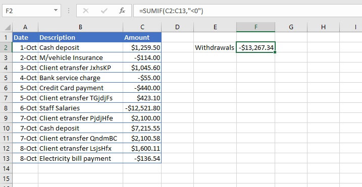
In the above formula, note the following:
- Only two arguments are required since the range is the group of cells where the values to be added are found. Therefore, the optional sum_range argument is omitted, and Excel sums the qualifying cells within the range.
- The criteria argument uses the logical expression “<0” to express values less than zero (withdrawals). The entire expression is enclosed within double quotes.
All arguments
By contrast, there are times when the range to be summed is not the same as the range where the qualifying values are located. An example is shown below.
Text criteria
In this example, we want to add all the sales made by the North team.
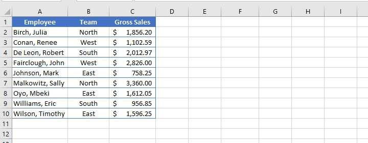 Obviously, the cells with the word “North” (column B) are not summable since they are all text values. Therefore the sum_range will be located elsewhere.
The range will be the group of cells (B2 to B10) where we will be looking to find the criteria (“North”). Once those are identified, we want to add the cells in the corresponding column C cells (sum_range).
In the output cell, we would enter:
=SUMIF(B2:B10,“north”,C2:C10) 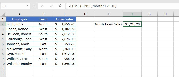 Here are some observations from the above:
- The equal sign (=) was omitted as this is understood by the SUMIF function. Entering =SUMIF(B2:B10,“=north”,C2:C10) would have yielded the same result. If used as part of the criteria, the equal sign must be included in the expression within double quotes.
- Text values are not case sensitive.
Cell reference criteria
In the following example, Excel looks within the range for the value in cell E2, and sums the corresponding values in column C.
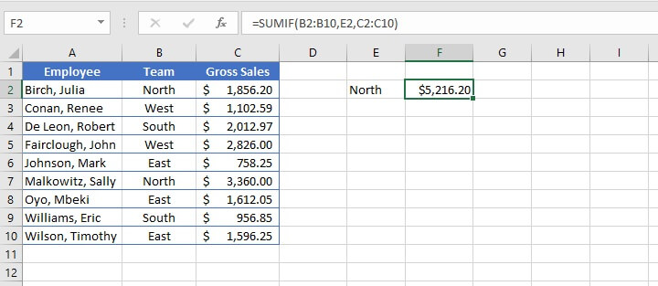 Note from the above example that there is no equal sign before the cell reference, as this is the default of the SUMIF function. Additionally, there are no quotation marks around the cell reference, as “E2” is not the literal value being extracted from the range.
Logical expression with cell reference
When using logical operators with cell references, the format is slightly different. In the example below, we can get the total sales made by the other teams, in other words, not equal to the North team. The operator <> is used to represent is not equal to.
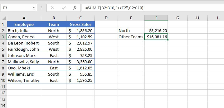 Since it is a logical operator, the logical operator “<>” is enclosed within double quotation marks, followed by an ampersand (&) to concatenate, or join, the operator to the relevant cell reference. Again there are no quotation marks around the cell reference since “E2” is not the literal value being extracted from the cell range.
Date criteria
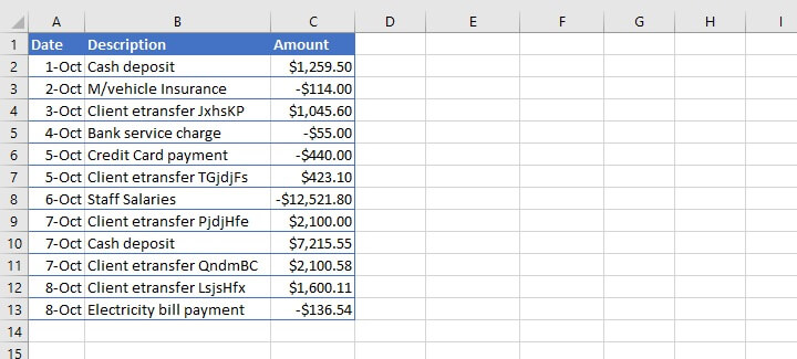
SUMIF can also be used with date criteria. To illustrate this, we can revert to our banking transactions example.
 Using the SUMIF function with logical operators, we can get the total value of all transactions that took place before a given date, such as October 3. The formula...
=SUMIF(A2:A13, “<10/03/2020”,C2:C13)...uses regional date settings for the explicit date format.
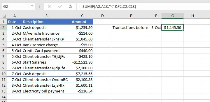
One disadvantage with this is that if the file is shared to a computer with different regional settings, it may result in the SUMIF formula searching for March 10 instead of October 3. It is therefore a better practice to enter the desired date in a cell, and then reference that cell in the SUMIF formula.
=SUMIF(A2:A13, “<”&F2, “C2:C13)...where the date value has been entered in cell F2.
Alternatively, the DATE function may be used.
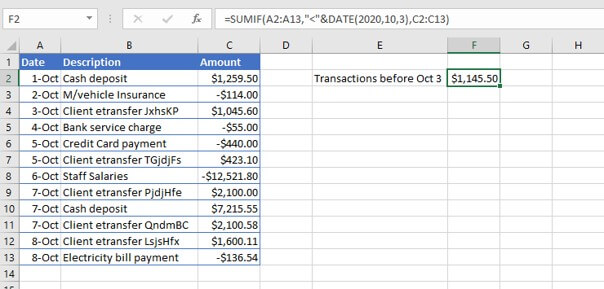 The < (less than) operator before a date represents earlier than, while the > (greater than) operator represents a date later than. An ampersand precedes the cell reference, but only the logical operator is enclosed by double quotation marks. Excel returns a value that calculates the sum of $1,259.50 and -$114.00.
SUMIF and wildcards
A common problem when looking to extract data is that the data we would like to group together is often similar, but not identical.
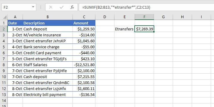
Let’s say we want to get the total value of all etransfer transactions below using SUMIF. We would not be able to simply use the word “etransfer” as a text criterion, since there are other characters in the cells, and they each have different transaction IDs.
Wildcards provide an excellent solution for this problem, and the SUMIF function does support the use of wildcards to accommodate partial matches.
| Wildcard | Meaning |
|---|---|
| * | Any number or string of unknown characters, or no character |
| ? | Any single unknown character |
| ~ | Precedes an asterisk or question mark to be used as a literal character |
The formula….
=SUMIF(B2:B13,“*etransfer*”,C2:C13)...will identify all cells within the range B2 to B13 which contain the word “etransfer” — whether or not any characters appeared before or after that word, and regardless of the number of characters.
Multiple Criteria
What about those times when the cells to be extracted from the range may satisfy any one of multiple criteria, like “apples” or “pears”?
Or what about cells that must satisfy more than one criteria, like greater than 500 and less than 1000?
SUMIF with OR logic
The first scenario is fairly easy to resolve. We can build two SUMIF formulas, and simply ask Excel to add their results by placing a plus sign (+) between them. In the example below, let us get the total number of apples and pears in stock.
=SUMIF(A2:A9, “*apples”,B2:B9)+SUMIF(A2:A9, “*pears”,B2:B9)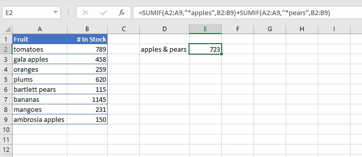
The first formula identifies cells in the range A2 to A9 that contain the word “apples” and sums the corresponding figure in column B (458 + 150).
The second formula identifies cells in the range A2 to A9 that contain the word “pears” and sums the corresponding figure in column B (115).
The grand total of 723 is displayed in cell E2.
For scenarios in which you want to know if at least one condition is true, check out our article on the OR function.
SUMIF with AND logic
Using SUMIF with an AND logic is somewhat less straightforward because we are seeking to isolate cells within a range that meet two or more conditions.
The problem is that the SUMIF function only works with one criterion at a time and the AND function only evaluates one cell at a time (it is unable to evaluate entire ranges), so they are incompatible. Therefore, the SUMIFS function exists to accommodate this type of scenario.
Useful SUMIF formats to remember
Here is a handy summary of the formats for the different types of criteria used with the SUMIF function.
| Criteria | Format example |
|---|---|
| Text value | =SUMIF(range, “apples”, sum_range) |
| Text value with unknown additional characters | =SUMIF(range, “*apple*”, sum_range) |
| Text value followed by a single unknown character | =SUMIF(range, “apple?”, sum_range) |
| Criteria which includes a literal question mark | =SUMIF(range, “what~?”, sum_range) |
| Numeric value | =SUMIF(range,500,[sum_range]) |
| Greater than or equal to numeric value | =SUMIF(range, “>=500”, [sum_range]) |
| Equal to cell reference | =SUMIF(range,D7,[sum_range]) |
| Not equal to value in cell reference | =SUMIF(range, “<>”&D7, [sum_range]) |
| Either one of multiple criteria | =SUMIF(range,criteria,[sum_range]) + SUMIF(range,criteria,[sum_range]) |
| Satisfies multiple criteria | use SUMIFS function |
Summary
We use the SUMIF Excel function to identify and find the sum of cells with a specific criterion within a range. It gives a single output and is therefore useful for summarizing data.
To learn more essential Excel functions and formulas, try our Microsoft Excel - Basic and Advanced course today. Or start with our free Excel in an Hour course for some formula basics.