
How to calculate averages in Excel
Believe it or not, there are many different kinds of averages, and different ways to go about calculating them. The following methods are covered in this resource:
AVERAGE function
The most universally accepted average is the arithmetic mean, and Excel uses the AVERAGE function to find it. The Excel AVERAGE function is used to generate a number that represents a typical value from a range, distribution, or list of numbers. It is calculated by adding all the numbers in the list, then dividing the total by the number of values within the list.
Syntax
The AVERAGE function in Excel is straightforward. The syntax is:
=AVERAGE(number1, [number2],...)Ranges or cell references may be used instead of explicit values.
The AVERAGE function can handle up to 255 arguments, each of which may be a value, cell reference, or range. Only one argument is required, but of course, if you’re using the AVERAGE function, it’s likely you have at least two.
AVERAGE calculates the statistical mean from a list of numbers. It ignores text and empties, but includes zeros.
The formula below will calculate the average of the numbers 100, 95, and 80.
=AVERAGE(100,95,80)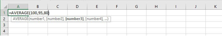
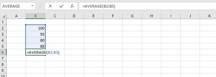
To calculate the average of values in cells B2, B3, B4, and B5 enter:
=AVERAGE(B2:B5)This can be typed directly into the cell or formula bar, or selected on the worksheet by selecting the first cell in the range, and dragging the mouse to the last cell in the range.
 In order to calculate the average of non-contiguous (non-adjacent) cells, simply hold the Control key (or Command key - Mac users) while making the selections.
If typing the cell references directly into the cell or formula bar, non-contiguous references are separated by commas. For example:
=AVERAGE(B2:B5,B8)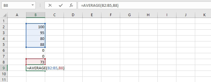
Download your free average in Excel practice file!
Use this free average in Excel file to practice along with the tutorial.
Remarks
When using the AVERAGE function, bear the following in mind.
- Text values and empty cells are ignored.
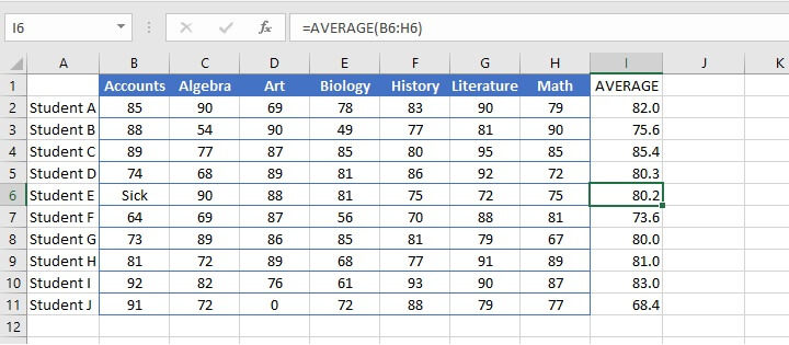
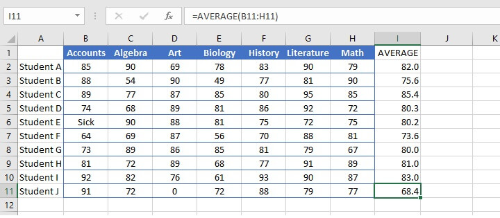
The word “Sick” in cell B6 (below) causes the AVERAGE function to ignore that cell altogether. This means that the average score in cell I6 was computed using the values in the range C8 to H8, and the total was divided by 6 subjects instead of 7.
- Zero values are included.
When determining the number of values to divide the total by, zeros are considered valid amounts and will therefore reduce the overall average of the distribution. Notice that Student J’s average is quite different from Student E’s average, even though their grade totals were similar.
AVERAGEA function
In order to eliminate this discrepancy, the AVERAGEA function may be used to include all values within a distribution, including text. The format is similar:
=AVERAGEA(value1, [value2],...)A range or cell references may be used instead of explicit values.
AVERAGEA evaluates text values as zero, while the logical value TRUE is evaluated as 1. The logical value FALSE is considered a zero.
AVERAGEA calculates the mean using all values within a list, including text. Text is treated as zero.
Compare the difference in results between using AVERAGE and AVERAGEA in the example below.
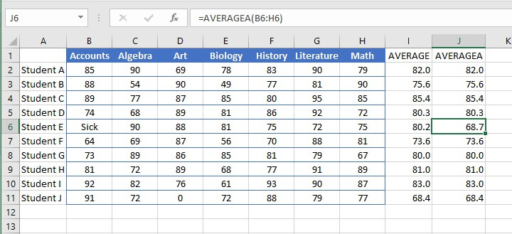 The averages for Student E and Student J are now similar when using the AVERAGEA function.
Check out the Microsoft Excel Basic & Advanced course
AVERAGEIF function
There are ways to find the average of only the numbers that satisfy certain criteria. With the AVERAGEIF function, Excel looks within the specified range for a stated condition, and then finds the arithmetic mean of the cells that meet that condition.
The syntax of the AVERAGEIF function is:
=AVERAGEIF(range,criteria,[average_range])- The range is the location where we can expect to find cells that meet the criteria.
- The criteria are the value or expression that Excel should look for within the range.
- Average_range is an optional argument. This is the range of cells where the values to be averaged are located. If the average_range is omitted, the range is used.
AVERAGEIF and AVERAGEIFS find the mean of only the values that satisfy certain criteria.
AVERAGEIF example 1
For example, from this list of various fruit prices, we can ask Excel to extract only the cells that say “apples” in column A, and find their average price from column B.


AVERAGEIF example 2
The criteria in an AVERAGEIF function may also be in the form of a logical expression, as in the example below:
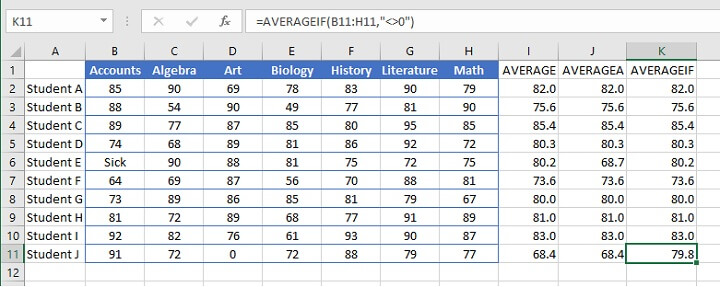
=AVERAGEIF(B4:H4,"<>0")The above formula will find the average of the values in the range B4 to H4 that are not equal to zero. Note that the third (optional) argument is omitted. Therefore, the cells in the range are used to calculate the average.
Since cells that are evaluated as zeros are omitted due to our criteria, notice the difference in Student E and J’s results below when using the AVERAGEIF function.
 In order to find the average of cells that satisfy multiple criteria, use the AVERAGEIFS function.
MEDIAN function
The arithmetic mean may be the most commonly used method of finding the average, but it is by no means the only one. One outcome of using the arithmetic mean is that it allows very high or very low numbers to sway the outcome, thereby significantly altering the results.
Take for example, the following list of numbers:
22, 1, 14, 21, 15, 16, 18, 100, 19, 19, 22, 25, 18
Finding the arithmetic mean would give a result of 23.8.
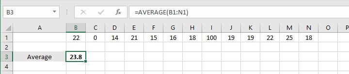 However, looking closely at the distribution of the numbers on the list, we would hardly say that 23.8 is the average value of those numbers. The problem, of course, is that the number 100 is an outlier and increased the sum of the numbers.
Therefore, in some situations, it is more desirable to use the MEDIAN function. This function determines the numerical order of the values being evaluated and uses the one in the middle as the average.
The syntax is:
=MEDIAN(number1, [number2], …)A range or cell references may be used instead of explicit values.
MEDIAN determines the numerical order of the list of values and uses the one in the middle as the average. Manual sorting is not necessary.
In the above example, the numerical order would be:
1, 14, 15, 16, 18, 18, 19, 19, 21, 22, 22, 25, 100
There are 13 numbers in the distribution, making the seventh number the middle value. Therefore, the median would be 19.
If the number of values is an even number, the median would be determined by finding the average of the two numbers in the middle of the distribution. So, for the values 7,9,9,11,14,15, the median would be (9+11)/2=10.
The MEDIAN function ignores cells that contain text, logical values, or no value.
MODE function
A third method for determining the average of a set of numbers is finding the mode, or the number that is repeated most often.
There are currently three “mode” functions within Excel. The classic, MODE, follows the syntax of:
=MODE(number1, [number2],...)In this function, Excel evaluates the values within the list or range, and selects the most frequently occurring number as the average value of the group.
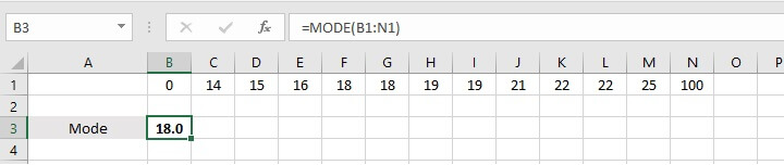
However, there are occasions when more than one number could be considered the mode. For example, consider the following list:
1, 14, 15, 16, 18, 18, 19, 19, 21, 22, 22, 25, 100
The numbers 18, 19, and 22 each appear two times. Which one is the mode? Excel chooses the first-appearing value as the mode — in the above case, 18.
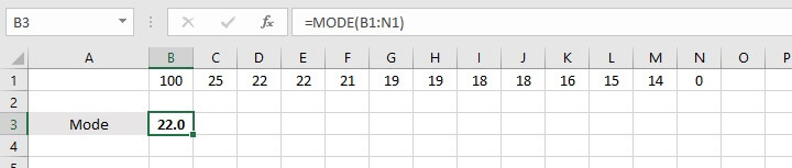
 If these same numbers were arranged in the reverse order, then 22 would be considered the mode.
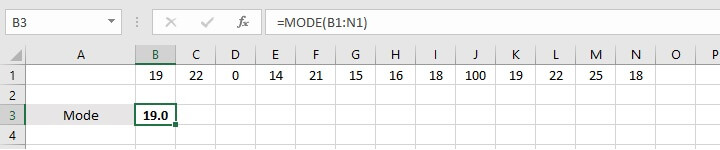
If the numbers were arranged in a random order, then Excel would select from 18, 19, and 22 based on whichever number appeared in the distribution first.
MODE uses the most frequently occurring number as the average value of the group.
For example, in the list:
19, 22, 1, 14, 21, 15, 16, 18, 100, 19, 22, 25, 18
The MODE function considers 19 as the mode.
MODE.MULT
The MODE.MULT function is a solution to the discrepancies experienced in the above scenario. It allows us to anticipate and account for the possibility that there may be more than one mode within a group of numbers.
The syntax is:
=MODE.MULT(number1, [number2],...)Since MODE.MULT is an array (CSE) function, these are the steps when using this function:
- Select a vertical range for the output
- Enter the MODE.MULT formula
- Simultaneously select Control + Shift + Enter
Pressing Control + Shift + Enter (CSE) together will cause Excel to automatically place braces (curly brackets) around the formula, and will return a “spill” of results equal to the number of cells selected in Step 1. If there is more than one mode, they will be displayed vertically in the output cells. The MODE.MULT function will return the “#N/A” error if:
- there are no duplicate values, or
- there are no additional modes in the output range.

MODE.SNGL
Like the MODE.MULT function, the MODE.SNGL function was rolled out with Excel 2010. The syntax is:
=MODE.SNGL(number1, [number2],...]The MODE.SNGL function behaves like the classic MODE function in determining the output.
Creative uses of the AVERAGE function
Top 3
We can combine the AVERAGE function with the LARGE function to determine the average of the top “n” number of values.
The LARGE function extracts the nth largest number from a range, using the format
=LARGE(array, k)where k is the nth number.
Using this format, we can display a number in the 1st, 2nd, 5th, or any rank.
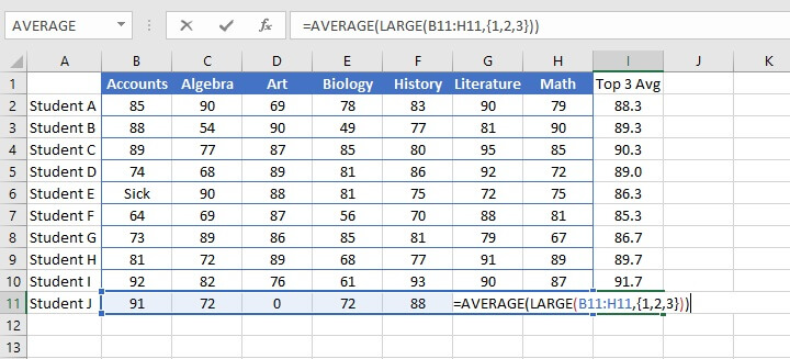
In order to get the average of the three largest numbers in a range, we would nest the AVERAGE and LARGE functions as follows:
=AVERAGE(LARGE(array, {1,2,3}))When we type braces around the k argument, Excel identifies the first, second, and third largest numbers in the array, and the AVERAGE function finds their average.
Bottom 3
We can use a similar logic to find the bottom 3 of a group of numbers using the SMALL function.
The following format will find the average of the three smallest numbers in the array.
=AVERAGE(SMALL(array, {1,2,3}))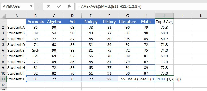
The three main methods of finding the average within Excel are the AVERAGE (mean), MEDIAN (middle), and MODE (frequency) functions. They are all easy to use, so choose the one that’s right for your type of data and the questions you want to answer.
Learn more Excel formulas and functions
To learn more useful formulas, functions, and real-world Excel skills, try the GoSkills Basic and Advanced Excel course.