
In Excel, there’s an easy way to identify and find the average of numbers that satisfy a certain criterion. With the AVERAGEIF function, Excel looks within the specified range for a single condition and then finds the arithmetic mean of the cells that meet that condition.
For more ways of calculating averages in Excel, check out our resources on calculating averages and weighted averages in Excel.
Syntax
The AVERAGEIF function has two required arguments and one optional argument.
The syntax is:
=AVERAGEIF(range,criteria,[average_range])- Range: the location where we can expect to find cells that meet the criteria.
- Criteria: the value or expression that Excel should look for within the range.
- Average_range: the optional argument. This is the actual range of cells where the values to be averaged are located. If the average_range is omitted, the range is used.
Download your free practice file!
Use this free Excel AVERAGEIF file to practice along with the tutorial.
Text criteria (all arguments)
For example, from the list of fruit prices below, we can ask Excel to extract only the cells that say “apples” in column A, and find their average price from column B. In this case, all three arguments are used, since the range does not contain the numbers being used to calculate the average price.
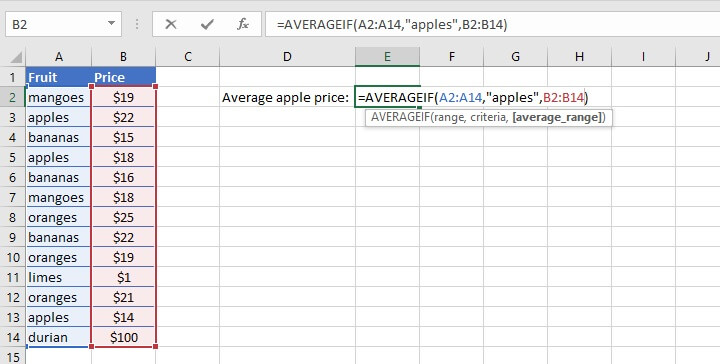
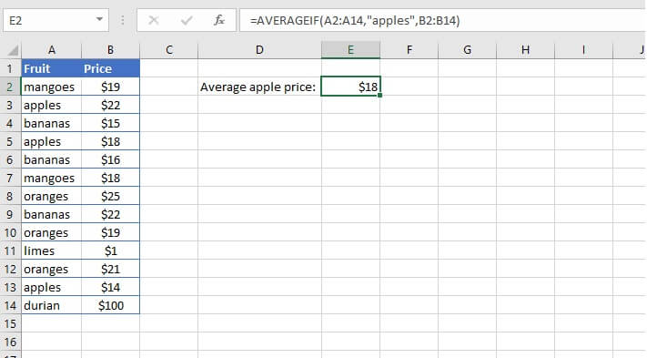 Note that the text value “apples” is placed within double quotes.
In cases where the range and average_range size or shape are different, Excel uses a combination of the first cell in average_range, plus the size and shape of the range, to determine the actual range of cells to be averaged.
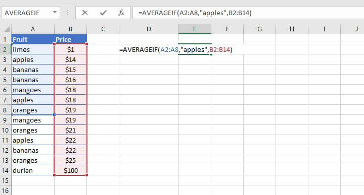
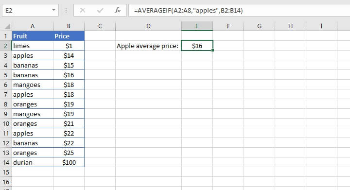 Though the average_range was stated as B2 to B14, only the cells in B2 to B8 were actually averaged, since those are the cells that corresponded with the A2 to A8 range.
Logical criteria
The criteria in an AVERAGEIF function may also be in the form of a logical statement, using the standard logical mathematical operators (=, >, <). However, as shown with the text examples above, the criteria argument defaults to “is equal to” so there’s no need to enter the equal sign (=) when stating the “is equal to” criterion.
The following combinations of these operators are also used for other specific logical comparisons.
| Operator | Meaning |
|---|---|
| >= | Greater than or equal to |
| <= | Less than or equal to |
| <> | Not equal to |
An example of a less than comparison is shown below. Note that the third (optional) argument is omitted. Therefore the cells in the range are used to calculate the average.
=AVERAGEIF(B2:H11, “<60”)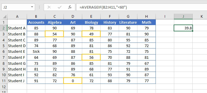 The formula above only takes into account and finds the average of the four highlighted values — 54, 49, 56, and 0. It ignores the “Sick” value in cell B6 since the AVERAGEIF function does not assign numeric values to text.
Cell reference criteria
We can also use a logical operator in combination with a cell reference to establish a criteria for the AVERAGEIF function. The following example finds the average of all cells within the range B2 to H11, which are less than the value in cell J1.
=AVERAGEIF(B2:H11, “<”&J1)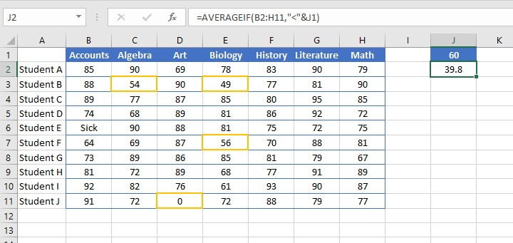 When using logical operators with cell reference criteria, the logical operator itself is enclosed within double quotation marks. This is followed by an ampersand (&) to concatenate, or join, the operator to the relevant cell reference.
As shown above, the text “Sick” in cell B6 was skipped when arriving at the average, so the only cells used in the calculation were C3, E3, F7, and D11.
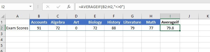
Cells not equal to
To exclude cells that contain a certain value, the <> (is not equal to) operator should be used. For example:
=AVERAGEIF(B2:H2,"<>0")The above formula will find the average of the values within the range B2 to H2 that are not equal to zero, that is, all cells within the range except D2 below.
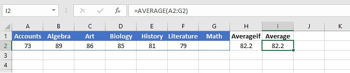
 By way of comparison, notice the result in the image below, where cell J2 uses the AVERAGE function instead.
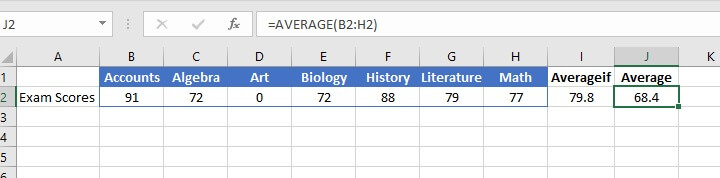 In the above example, the AVERAGE function is used in cell J2, which means all values in the range B2 to H2 are used to calculate the range. Therefore, the zero value in cell D2 affects the outcome of the average.
If not blank
The AVERAGE function ignores blank cells, so the AVERAGEIF function isn’t needed if we want to get the average of cells that are not blank. To prove this point, we created a complex AVERAGEIF formula by using the logical operator <> together with empty double quotes, to represent the criterion is not equal to an empty cell in the example below.
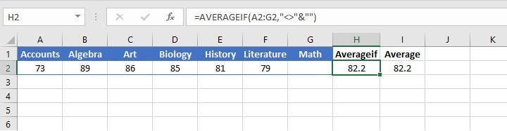
 The average calculated by the AVERAGEIF function in cell H2 is identical to that calculated by the AVERAGE function in cell I2. It makes sense to use the AVERAGE function for cells that are not blank — it’s the simplest and least complicated solution.
Multiple criteria
AVERAGEIF with OR logic
There may be times when we’d like to find the average of cells within a range that satisfies any one of multiple criteria (like “apples” or “oranges”). This scenario is fairly easy to resolve by incorporating OR logic.
We can build an AVERAGEIF formula that finds the average price of “apples” and one that finds the average price of “oranges” — and simply ask Excel to average their results by nesting the two AVERAGEIF functions into the AVERAGE function, as shown below.
=AVERAGE(AVERAGEIF(A2:A14,"apples",B2:B14),AVERAGEIF(A2:A14,"oranges",B2:B14))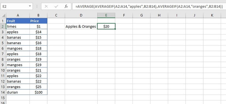
AVERAGEIF with AND logic
In order to find the average of cells that satisfy multiple criteria (such as “greater than x but less than y”), we would use the AVERAGEIFS function, which combines AVERAGEIF with AND logic. This identifies and finds the average of cells that satisfy all of the stated criteria.
AVERAGEIF with partial matches
Sometimes the cells we want to extract from a range are alike in some ways, but they aren’t identical. In other words, they are only a partial match. Wildcards provide a great solution for identifying these cells, and AVERAGEIF does work with wildcards.
| Wildcard | Meaning |
|---|---|
| * | Any number or string of unknown characters, or no character |
| ? | A single unknown character |
| ~ | Precedes an asterisk or question mark to be used as a literal character |
We can find the average of all text in the range A2 to A14 that ends with “es” by placing an asterisk before “es” as our criteria.
=AVERAGEIF(A2:A14,"*es",B2:B14)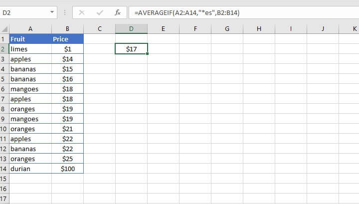 The result of the above criteria is that the average price of limes, apples, mangoes, and oranges is calculated and returned in cell D2.
Points to watch for
- If you get a #DIV/0! error, it means that Excel wasn't able to find a value within the range that satisfies the specified criteria.
- AVERAGEIF ignores cells within the range that contain the Boolean values TRUE or FALSE.
To learn even more ways of calculating averages in Excel, check out our resources on calculating averages and weighted averages in Excel.
Ready to be an Excel pro? You can start with the free Excel in an Hour course today then explore our other Excel courses including the Microsoft Excel - Basic and Advanced course.