How to Use the Excel FIND Function

---

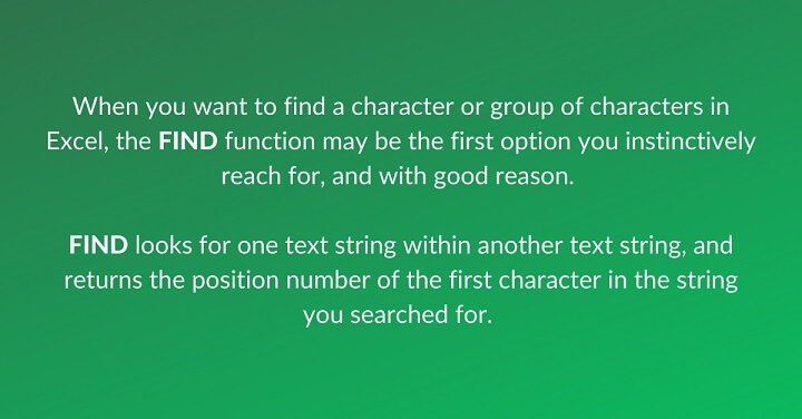
When you want to find a character or group of characters in Excel, the Excel FIND function may be the first option you instinctively reach for, and with good reason.

FIND looks for one text string within another text string and returns the position number of the first character in the string you searched for. 

Below are a few pointers to bear in mind and some tips for working with the Excel FIND function.

Syntax

The syntax of the FIND function is as follows:

=FIND(find_text,within_text,[start_num])

• Find_text is the substring or character you want to locate.
• Within_text is the cell reference or text string within which you will look for your character(s).
• Start_num (optional argument) is the position number of the character where your search should begin. If this argument is omitted, FIND starts looking from the first character of the string.

Remarks

• Arguments that are stated as explicit text should be placed inside double quotation marks.
• Arguments that are stated as cell references must not be placed inside double quotes.
• The FIND function is case-sensitive. If you’d like to perform a non-case-sensitive search, the SEARCH function is a better choice.
• FIND does not support the use of wildcards. However, the SEARCH function does.
• If no match is found, FIND returns a #VALUE! error.

---

---

Basic application

Here is a simple example of how we might use the FIND function.

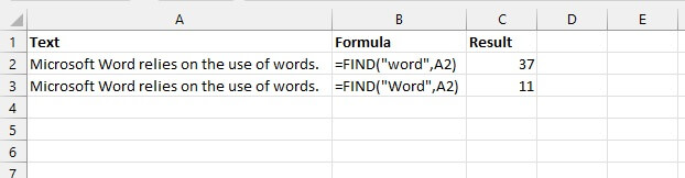In cells A2 and A3, the substrings “Word” and “word” occur in a single text string. Since FIND is case sensitive, a find_text argument of “word” results in the formula skipping the “Word” substring and locating “word” at the 37th position. By changing find_text to “Word” Excel returns a value of 11.

Instead of using an explicit text string as the find_text argument, we may use a cell reference to determine if a cell in Excel contains a particular word or group of characters.

=FIND(B2,A2)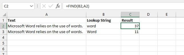

The formula in cell C3 is:

=FIND(B3,A3)

Note that when using cell references, we do not use double quotation marks since we are not trying to find the literal value “B2” or “B3”.

Other than the differences in the use of wildcards and case sensitivity, the FIND function works in essentially the same way as SEARCH. It is often combined with other Excel functions to solve practical problems. 

Combining FIND with other functions

FIND can be combined with other Excel text functions like LEN, TRIM, SUBSTITUTE, REPLACE, LEFT, RIGHT, and MID to extract, split or replace specific elements from text strings. The original text and/or the desired output may be of either fixed or variable length. Those of variable length usually require a bit of creative thinking, so it’s useful to know the type of value returned for each function in order to determine the combination that will give the result you want. 

A summary of these functions is shown below.

Replace a substring if present

FIND is often embedded within the REPLACE function to find a substring inside another one and then replace it with something else. The syntax of the REPLACE function is:

=REPLACE(old_text, start_num, num_chars,new_text)

• Old_text is the full text string that contains the substring to be replaced.
• Start_num is the starting position number of the text to be replaced.
• Num_chars is the length of the text to be replaced. 
• New_text is the text that will replace the characters being removed.

Below, we might want to find the word “song” and replace it with the word “poem” if it is present.

=REPLACE(A2,FIND("song",A2),4,"poem")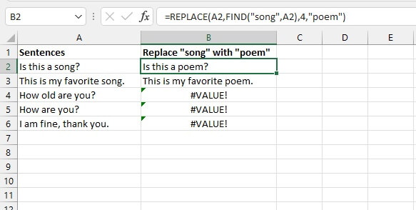

Since the exact location of the “song” substring within the text string is unknown, the position number returned as a result of the FIND formula was used as the start_num argument of the REPLACE function. With this formula, cells that did not contain the substring returned a #VALUE! error. This can be avoided by adding the IFERROR function to return an alternative result.

The syntax of the IFERROR function is:

=IFERROR(value, value_if_error)

By using the REPLACE/FIND formula combination as the value argument of the IFERROR function, Excel evaluates whether an attempt to find the substring results in an error.

=IFERROR(REPLACE(A2,FIND("song",A2),4,"poem"),A2)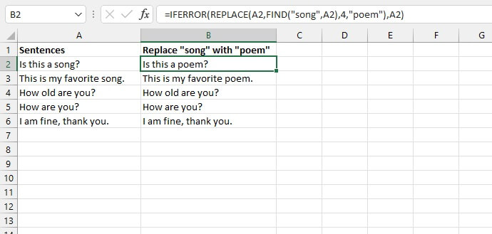

That last argument in the function above is set to return the text in the Column A cell if no match is found by the FIND argument.

Extract a portion of text from a larger text string

The FIND function is often combined with the LEFT, RIGHT, and MID functions to extract a portion of text by using its position number within a larger text string.

Extract leftmost characters

To extract usernames from the following email addresses, we can use the FIND function as an argument of the LEFT function.

The LEFT function begins counting from the leftmost character. There is an optional argument to extract several characters at a time. If that argument is omitted, only a single character is extracted. The syntax of the LEFT function is:

=LEFT(text, [num_chars])

Since the FIND function returns the position number of a character or text string, the result of the FIND function can be used as the num_chars argument of the LEFT function. We typically subtract 1 from that result to get the “stop” position of the string we want to extract.

=LEFT(A2,FIND(“@”,A2)-1)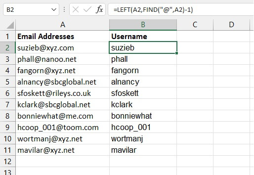

The result of this FIND formula becomes the num_chars argument of the LEFT formula.

Extract rightmost characters

To extract the domain name from the email addresses, we could either use the RIGHT and LEN functions together. Or, with a little creativity, the MID function. See both options below.

Option 1

The LEN function counts the number of characters that are in a text string. The syntax is:

=LEN(text)

The RIGHT function starts counting from the rightmost character and returns counting from the rightmost character. The syntax is as follows:

=RIGHT(text, [num_chars])

Therefore we can use the previous LEN/FIND formula combination as the num_chars argument of the RIGHT formula.

=RIGHT(A2,LEN(A2)-FIND("@",A2))

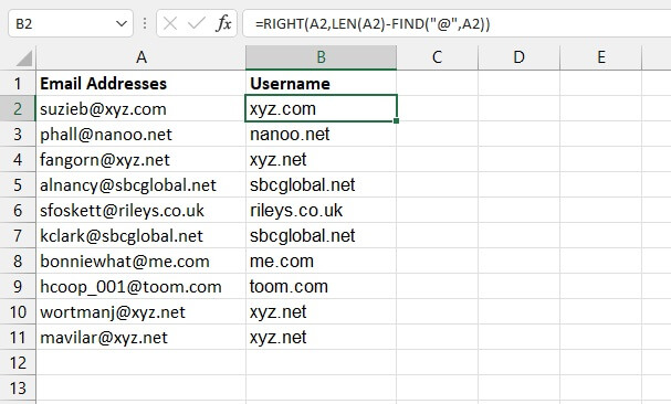The above formula uses FIND to get the position number of the “@” symbol. It subtracts that from the length of the original string, which is then used as the num_chars argument of the RIGHT function.

Option 2

The second option is even easier. The MID function can grab characters from the middle of a text string all the way to the end. The syntax is:

=MID(text, start_num, num_chars)

All the arguments are required. MID allows us to treat a substring from anywhere in the text all the way to the end as a middle string by specifying a number that we are sure is larger than the length of the text string. In this example, we’ll use 100. 

=MID(A2,FIND(“@”,A2)+1,100)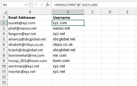

Adding 1 to the position number of the “@” character tells us the starting position (or start_num) of the MID function.

Determine if a substring is present

FIND can be nested with the ISNUMBER function to test whether a particular substring is present or not. The way this works is that if FIND returns a position number, then the ISNUMBER formula will return a value of TRUE. And if FIND returns a #VALUE! error, ISNUMBER will return FALSE.

The syntax of the ISNUMBER function is:

=ISNUMBER(value)

So we can use the FIND formula as the argument of the ISNUMBER formula.

=ISNUMBER(FIND(“xyz.net”,A2))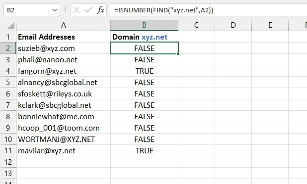

The above formula evaluates whether each text string contains the substring “xyz.net”. If it does not, the formula returns a value of FALSE. Note that in the example above, the formula referring to cells A4 and A11 returned TRUE, while the one referring to A10 returned FALSE since FIND is case-sensitive. When the case does not matter, it’s better to use the SEARCH function.

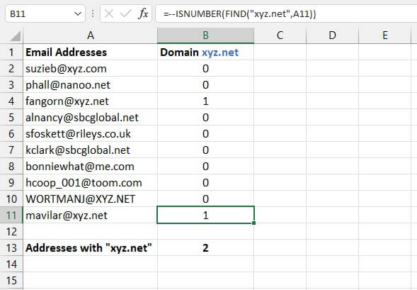
For a simple way to count the number of instances of a TRUE result, place two minus signs before the ISNUMBER function. This will cause the formula to return 1 or 0 for TRUE or FALSE, respectively. These results can be used with the SUM function to add the number of addresses that have a “xyz.net” domain.

=--ISNUMBER(FIND(“xyz.net”,A11))

We can take this one step further by returning customized responses using the IF function. 

The IF function evaluates a logical statement and returns one response if the statement is TRUE and a different response if the statement evaluates to FALSE. With this principle, we can tell Excel what it should do if ISNUMBER returns a TRUE response and what it should do if it doesn’t.

The syntax of the IF function is:

=IF(logical_test, [value_if_true], [value_if_false])

So we can make our ISNUMBER/FIND formula combination the first argument of the IF formula.

=IF(ISNUMBER(FIND(2,A2,5)),"Yes","No")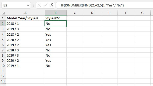

In the example above, we used all three arguments of the FIND function. This allowed us to find the value “2” starting with the 5th value. 

The optional start_num argument is usually used when the substring being searched for appears more than once, and we’d like to ignore a certain number of initial occurrences. In this case, when we specify the start number, we get FIND to ignore the digits in the year. 

Beginning with the 5th character, if the number “2” is found, the FIND function returns the position number, resulting in a TRUE output by the ISNUMBER function. The IF function is nested around this so that if the cell does contain the desired text, then “Yes” is returned for TRUE results and “No” for FALSE results.

Note: Searching for a numeric value works with (or without) the double quotes.

FIND vs. FINDB

If you’re interested in learning about the FINDB function, note that the only difference between FIND and FINDB is that FINDB counts 2 bytes per character when a double-byte character set (DBCS) language is set as the default language. The languages that support DBCS include Korean, Japanese, Chinese (Simplified), and Chinese (Traditional).

Otherwise, FINDB behaves the same as FIND, counting 1 byte for each character. For this reason, we have only discussed FIND in this resource.

Other ways to find things in Excel

The Excel FIND function helps you look for something within a specific text string. But if you want to look up an item within an Excel table or data set, the VLOOKUP or HLOOKUP functions might be more suited to that task. 

If you have Excel 365, you’ll find that XLOOKUP is even more flexible. It can do everything the previous functions can and even more. 

If you prefer non-formula methods to locate text in Excel, click here to learn how to find and replace a text string with another text string.

Explore our course library to learn about other Excel tools. Try the Microsoft Excel - Basic and Advanced course.

Level up your Excel skills

Become a certified Excel ninja with GoSkills bite-sized courses

Start free trial