12 Basic Excel Formulas You Need to Know

So you’re getting started in Excel and you’ve heard about how great formulas are. There’s just one thing — you don’t know much about how to use Excel formulas. Forget complex stuff like the PI function in Excel; the basics can be confusing too!

Let’s fix that right now. As a bonus, we’ve also put together our list of the 12 best basic Excel formulas.

---

---

What are formulas used for in Excel?

Formulas are what take Excel from being a plain spreadsheet to being a productivity tool. They are mathematical expressions that simplify and, at times, automate mathematical and logical operations so that we can solve problems and analyze data. 

Excel interprets a formula as a command to do a calculation using one or more of the basic math operations —  addition, subtraction, multiplication, and division. 

These operations are represented by the plus, minus, asterisk, and forward slash (+, -, *, /) symbols, respectively. To signal that a calculation is expected, always start an Excel formula with an equal (=) sign.

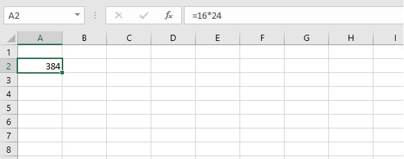
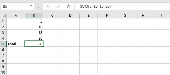
So, this is a formula:

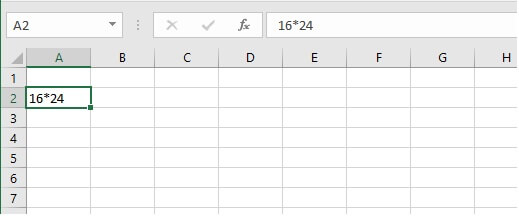
But this isn’t a formula:

What’s the difference between formulas and functions?

Functions are Excel-defined formulas. They are Excel’s way of allowing you to quickly perform complicated or frequently-used formulas without having to build the task yourself step by step. 

Since functions are actually formulas, they also begin with an equal sign, but the most recognizable thing about functions is that they have friendly names defined within Excel. 

The names of these functions are meant to be easy to remember by being close to the action they perform. For instance, there’s the SUM function to add values, the LOWER function to convert text to lowercase, and the COUNTBLANK function that counts the number of empty cells within a range.

Each function has arguments or values that should be stated in a particular order. Once valid arguments are provided in the correct format, Excel performs the calculation and displays the result in the cell where the formula was entered.

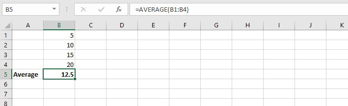
For example, here’s how to find the average or mean of a group of numbers. We can enter a formula by adding the numbers using the plus (+) symbol, then, using the forward slash (/), dividing that total by the number of values within the data set. However, instead of performing these steps, a pre-built AVERAGE function exists in Excel to perform this task with very little effort on your part.

Function syntax and return value

Excel functions have a syntax or a format that they must follow in order to be considered valid.

All functions have the following general structure:

equal sign > function name > open parenthesis > arguments > close parenthesis

For example, to find the average of values in cells A2 to A10, the AVERAGE formula would be written in the following way:

=AVERAGE(A2:A10)

While entering your function, Excel helps you along in the following ways:

• By suggesting a list of functions that start with the letters you’ve typed in. If you press the tab key, Excel will complete the name of the first function on the list, and the open parenthesis. Or you can arrow down to the one you want, press the Tab key, and finish up by entering the arguments and closed parenthesis.
• By prompting with the name of the next argument in the sequence.
• By distinguishing between required and optional arguments. Optional arguments are shown in square brackets.

Different methods to insert formulas 

Excel uses the equal symbol to recognize formulas (and by extension, functions). 

1. Using explicit numbers

To enter a non-function formula in Excel, type an equal sign, then the equation using the standard mathematical operators and numeric values and/or cell references.

=7+2*2

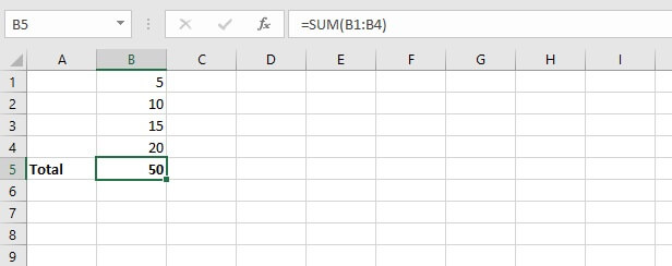
2. Using cell references

The same result can be achieved by entering the cell references that contain the values you want to use in your formula. 

=A7+A8*A8

The cell referencing method is usually more efficient, especially in cases where multiple formulas make reference to the same cell. Since you can quickly update the source value, the dependent cells containing the formulas will be recalculated and updated immediately.

Note:

• Excel follows the PEMDAS (Parentheses – Exponents – Multiplication – Division – Addition – Subtraction) order of operations rule. This means that values within parentheses will be processed first, followed by exponents, and so on.

Different methods to insert functions

Excel has more than 400 functions that can be accessed in any of the following three ways:

1. If you already know the function name, just type it directly into the cell where you would like to see the result displayed, led of course by an equal sign.
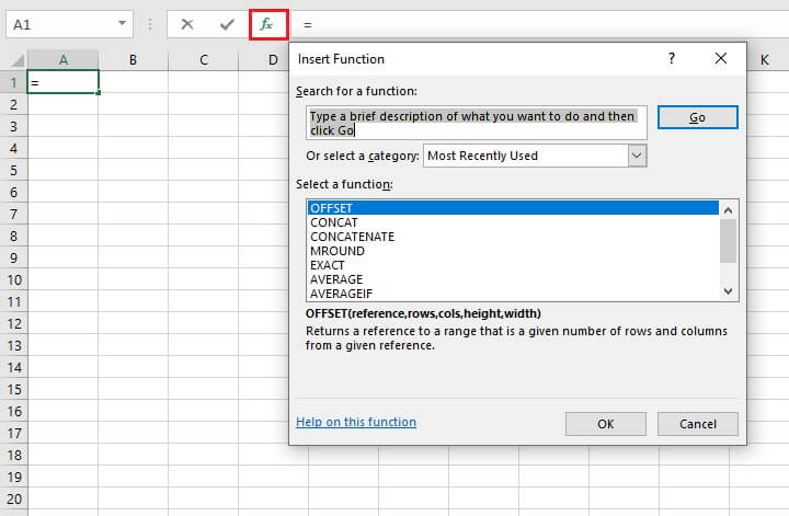
2. Use the Insert Function button to the left of the Formula Bar. Use the 'Insert Function' dialog box to search for or select a function from a category. 

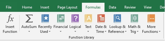
3. You may also use the Formulas tab to select a function by category.

Methods 2 and 3 have the advantage of defining each argument and giving a preview of the result while the values or cell references are being entered. 

12 basic Excel functions you need to know

Below is a list of 12 Excel functions we highly recommend because of how frequently they’re used, because of their usefulness in executing complex tasks, or because they are the basis for other functions.

1. SUM

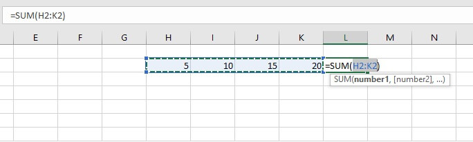
The SUM function adds values. You can add explicit numerical values, cell references, ranges, or a mix of all three. The basic syntax is:

SUM(number1, [number2], [number3]...)

Note that arguments are separated by commas. A space may also be inserted or may be omitted.

SUM is usually the first function one learns in Excel, and it’s a good example of how Excel can save time by reducing keystrokes. While the operation of adding values is, of itself, quite uncomplicated, it is the act of entering the values themselves that tends to be time-consuming. 

By allowing the use of cell ranges instead of values, you eliminate having to enter each value one by one as you would on a calculator.  

Here’s a handy tip: If you want to quickly sum values in a contiguous (unbroken) range, go to the very next cell and click the Autosum icon on the Home tab. Excel will insert the SUM function to find the total of all the previous cells that contain numeric values. 

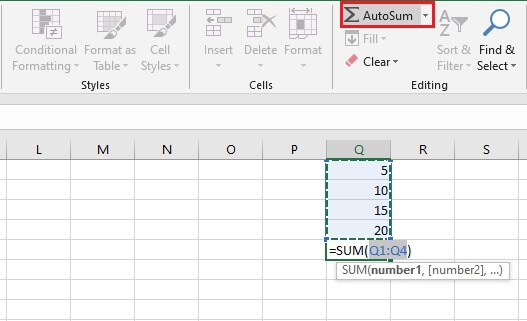The Alt = shortcut also accomplishes this.

2. AVERAGE

Another basic arithmetic calculation that Excel takes care of is the AVERAGE function. As seen before, it eliminates the need to perform a two-step calculation and is, therefore, one of our recommended basic functions.

The syntax of the AVERAGE function is:

AVERAGE(number1, [number2], ….)

Arguments may also be entered as a cell range.

But what if you want to find an average that isn’t the arithmetic mean? For instance, maybe you want to know the mode or the median of a set of numbers. Check out this resource on averages to learn about these functions.

3. IF

The IF function ventures into the realm of logical functions. Logical functions basically test whether a situation is true or false. The IF function takes it a step further by performing one action if the situation is true, and another action if it is false.  This function is a great example of how Excel can turn a plain data sheet into an analytical tool.

The situation tested may be where one value or statement is equal to, greater than, or less than another value or statement.

The syntax of the IF function is:

IF(logical_test, [value_if_true], [value_if_false])

• Logical_test is the statement to be tested.
• Value_if_true is the value or expression Excel should return if the cell passes the logical test.
• Value_if_false is the value or expression Excel should return if the logical test fails.

In the case of the IF function, if the value_if_true is omitted, the value_if_false must be stated, and vice versa. But both cannot be omitted.

With IF, we can get Excel to perform a different calculation or display a different value depending on the outcome of a logical test. The IF function asks you for the logical test to perform, what action to take if the test is true, and an alternative action if the result of the test is false.

Though both the second and third arguments are declared as optional, at least one of those arguments must be provided.

=IF(B2>=90,“Outstanding”, “”)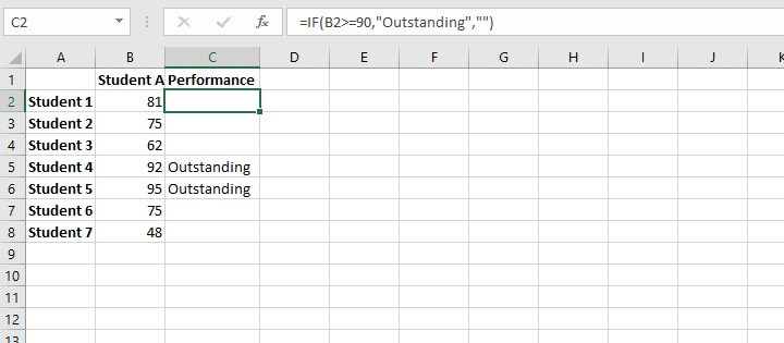

The formula above tests whether the value in cell B2 is greater than or equal to 90. If it is, Excel returns the text value “Outstanding” (note that text values are entered between double quotes). 

If the value is not greater than or equal to 90, the cell should remain blank (note the empty double quotation marks). This formula is then copied to cells C3 to C8, where C3 evaluates the value in B3, and so on.

To learn more about relative cell references and how they help when copying formulas, check out this resource (Relative References in Excel - A Beginner's Guide).

4. SUMIFS

SUMIFS is a very useful Excel function. It combines the basic SUM operation with an IF logical test to add only cells that meet multiple user-defined criteria. 

Up to 127 pairs of criteria may be submitted. Cells that are considered a “match” or “qualifying” would need to satisfy all the stated criteria. SUMIFS is superior to the SUMIF function, which is limited to only one condition being evaluated at a time.

The SUMIFS syntax is:

SUMIFS(sum_range, criteria_range1, criteria1, [criteria_range2], [criteria2],...)

• Sum_range - is the range of cells to sum.
• Criteria_range1 - is the range of cells to be evaluated.
• Criteria1 - is the condition that cells in criteria_range1 must satisfy.
• Criteria_range2 - is the second range of cells to be evaluated.
• Criteria2 - is the condition or criterion that cells in criteria_range2 must satisfy.

All arguments after criteria1 are optional. 

Here is an example of SUMIFS at work.

=SUMIFS($C$2:$C$10,$B$2:$B$10,E2)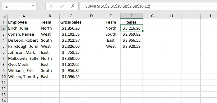

Note the use of absolute cell references above to lock the cell ranges. This prevents shifting of the range when the formula is copied to other cells.

5. COUNTIFS

The COUNTIFS function is another member of the IF family of functions. It counts only cells that satisfy all the stated criteria. COUNTIFS is superior to the COUNTIF function, which allows only one condition to be evaluated at a time.

The syntax of the COUNTIFS function is:

COUNTIFS(criteria_range1, criteria1, [criteria_range2, criteria2]…)

• Criteria_range1 - is the first range to be evaluated.
• Criteria1 - is the first criterion that cells in criteria_range1 must satisfy.
• Criteria_range2 - is the second range to be evaluated.
• Criteria2 - is the first criterion that cells in criteria_range2 must satisfy.

All pairs after criteria1 are optional. Up to 127 range and criteria pairs are allowed.

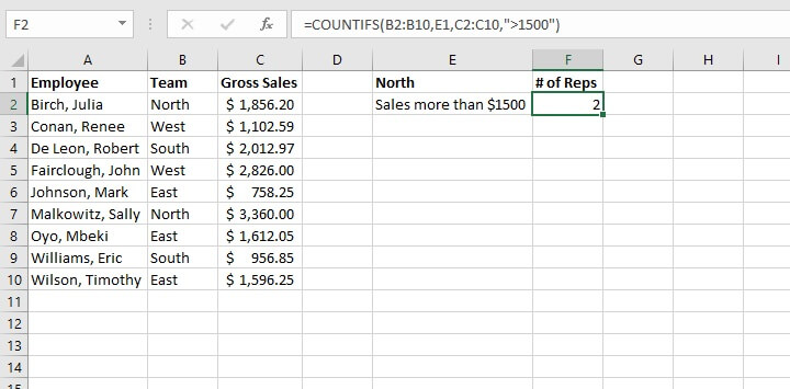
To count the number of sales reps on the North team who achieved more than $1,500 in sales, the formula would be:

=COUNTIFS(B2:B10,E1,C2:C10,E2)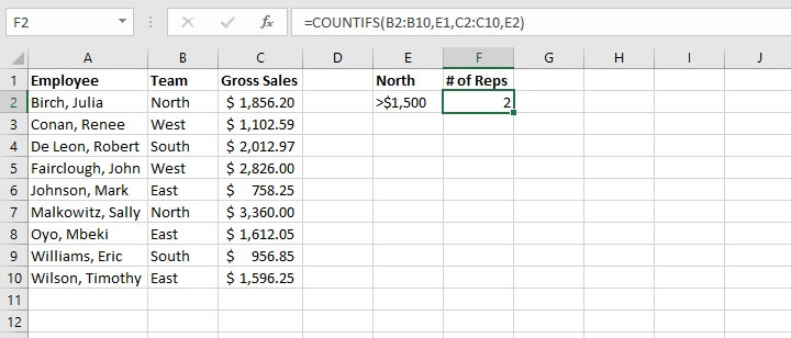

Note: In general, text values in COUNTIFS need to be enclosed in double quotes (""), and numbers do not. But when a logical operator (> or <) is used with a number, both the number and operator must be enclosed in quotation marks. 

=COUNTIFS(B2:B10,E1,C2:C10,“>1500”)

6. VLOOKUP

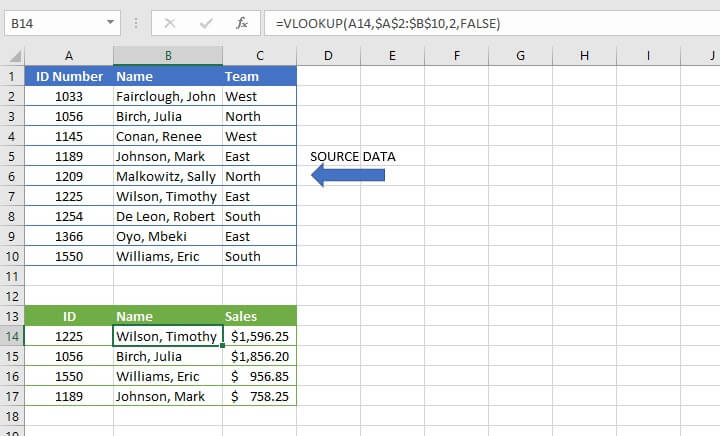
The VLOOKUP function will be a game-changer once you start using it. Use VLOOKUP when you need to find things in a table or an array. VLOOKUP is used in many search-type situations, for example, to find an employee name based on their employee ID.

The VLOOKUP syntax is:

VLOOKUP(lookup_value, table_array, col_index_num, [range_lookup])

Here’s what those arguments mean:

• Lookup_value - is what you want to look up. 
• Table_array - where you want to look for it.
• Col_index_num - is the column number in the range containing the value to return. 
• Range_lookup - type TRUE for an approximate match, or FALSE for exact match.

The formula

=VLOOKUP(A14,$A$2:$B$10,2,FALSE)

is entered in cell B14, which returns the name of the employee matching the ID number.

In recent years, VLOOKUP has been outperformed by XLOOKUP, which is more flexible and arguably easier to use. XLOOKUP is available in Microsoft 365 and later.

7. COUNT

The COUNT function will count the number of cells that contain numbers. You can use this function to get the number of entries in a number field that’s in a range or an array of numbers. The syntax of the COUNT function is:

=COUNT(value1, [value2]...)

Placing the COUNT function in cell B6 below determines that there are three numeric values between cell B1 and B5.

=COUNT(B1:B5)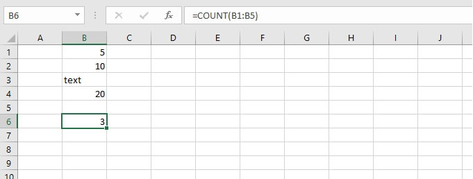

8. TRIM

The TRIM function will remove all spaces from text except for the single spaces between words. TRIM is often used on text imported from another application that may have irregular spacing.

Follow this simple format:

=TRIM(text)

TRIM works on a text string entered within double quotes, or a single cell reference.

=TRIM(A1)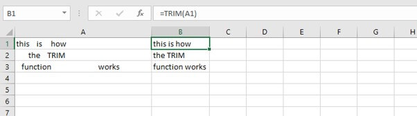

9. LEFT 

The LEFT function is used to extract a specific number of characters from a text string, such as a specific portion of a telephone number. The syntax of the LEFT function is:

=LEFT(text, [num_chars])

Num_chars refers to the number of characters to be extracted counting from the left. If the num_chars argument is omitted, Excel returns the leftmost character only.

=LEFT(A2,3)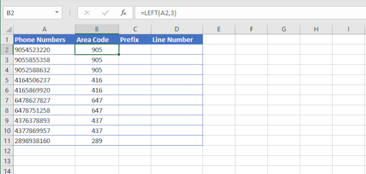

10. RIGHT 

The RIGHT function is used to extract a specific number of characters from a text string, such as a specific portion of a telephone number. The syntax of the RIGHT function is:

=RIGHT(text, [num_chars])

Num_chars refers to the number of characters to be extracted counting from the right. If the num_chars argument is omitted, Excel returns the rightmost character only.

=RIGHT(A2, 4)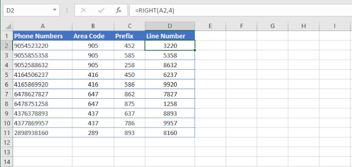

11. MID

The MID function is used to extract text from the middle of a text string. The syntax of the MID function is:

=MID(text, start_num, num_chars)

The start_num argument tells Excel what position number to start extracting from (counting from the left), while num_chars tells it how many characters to extract.

=MID(A2,4,3)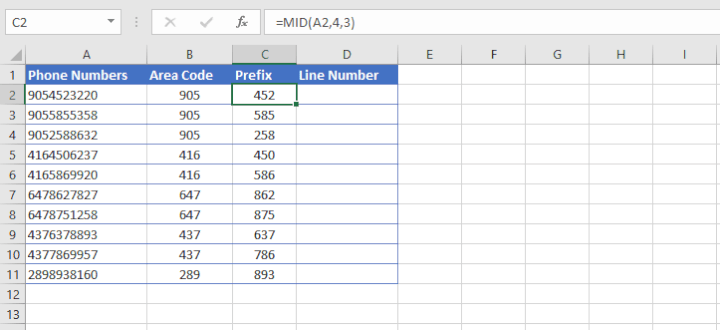

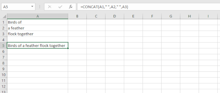
12. CONCAT

Our final basic Excel function is CONCAT. This function combines the values from multiple cells into one. This is useful for piecing together the different parts of text, for example, to combine a first name and last name into a full name. The syntax is:

=COUNT(text1, [text2], [text3]...)

To insert delimiters (such as a space, dash, or comma) simply enter that bit of text as one of the text arguments within double quotes.

For example:

=CONCAT(A1," ",A2," ",A3)

will copy the value from cells A2 and B2, inserting a space between them. 

Conclusion - basic Excel formulas

And that's our top 12 Excel formulas list! Download the practice file and think about situations where you might use these functions at work. 

Don’t forget to try one of our Excel courses to learn some valuable Excel skills. You can try the free Excel in an Hour course, but if you really want to ramp up your formula knowledge, we suggest the Excel Basic and Advanced course.

Level up your Excel skills

Become a certified Excel ninja with GoSkills bite-sized courses

Start free trial