How to Use the Excel MID Function

Three of the most popular text functions in Excel are MID, LEFT, and RIGHT. They are all used to extract a piece of text from a string. As its name suggests, MID is specifically used to extract a substring that is bounded by characters on each side.

The MID function has three arguments, and they are all required.

Syntax and arguments

MID(text, start_num, num_chars)

• Text is the original text string from which the data will be extracted
• Start_num is the position number of the first character to be extracted, counting from the leftmost character
• Num_chars is the number of characters to be extracted

Remarks

There are a couple of points to bear in mind about MID before we can start using it to solve problems.

1. Like its siblings LEFT and RIGHT, the MID function returns values formatted as Text. This means that even if the values extracted are numeric values, Excel will store them as text. This can be a problem if you want to do a mathematical calculation with your extracted values later. Click here to learn how to fix that. 
2. Start_num must be greater than or equal to 1. Otherwise, Excel will return a #VALUE! error.

Basic application

At its most basic usage, the MID function is used for strings of a fixed length. At the very least, the position number of the first character to be extracted as well as the length of the desired substring are both known.

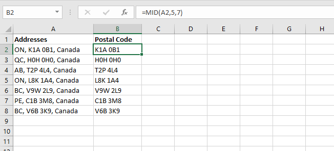
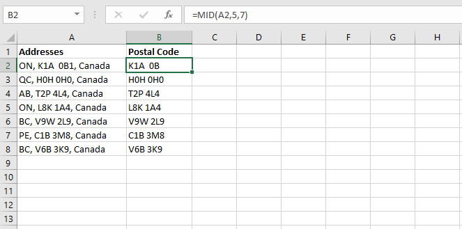
Below is a simple example of how to use the MID function in Excel. Note that the format of the province code, postal code, and country name are consistent for each cell in Column A. With this information, it’s pretty easy to pull the postal code only from the original string.

=MID(A2,5,7)

Extract text starting with the n^th character

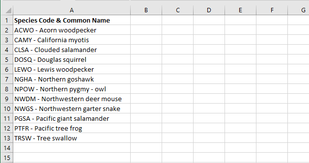
If you have a dataset with text of variable lengths where you would like to drop the leading “X” number of characters, this is pretty easy too.

In the example below, the common name of each species starts with the 8th character, but the length of the string is not fixed. 

Since MID requires the third argument, we can’t just leave it blank. We have a choice here. 

• We can either find the length of the string using the LEN function and then use that to tell MID how many characters will need to be extracted. We would end up with a formula like this:

=MID(A2,8,LEN(A2)-7)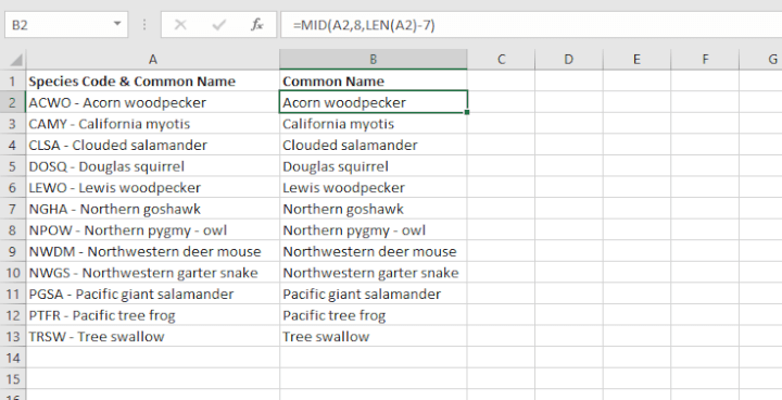

That would certainly work, but in this case, it really isn’t necessary. 

• Our second option is as follows. It is useful to know that MID allows us to treat the entire string after the dash as a middle string by specifying a number that is very large. For the sake of this example, we can use 100. 

=MID(A2,8,100)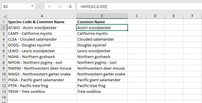

And that neatly takes care of that.

Combining MID with other functions

Quite often, MID is often combined with other Excel text string functions like LEN, TRIM, SUBSTITUTE, LEFT, RIGHT, FIND, and SEARCH to split data or to extract specific elements from text strings. The original text and/or the desired output may be of either fixed or variable length. Those of variable length usually require a bit of creative thinking, so it’s useful to know the type of value returned for each function in order to determine the combination that will give the result you want. A summary of these functions is shown below.

Function	Syntax	Return value
LEN	LEN(text)	Number of characters
TRIM	TRIM(text)	Text without leading and trailing spaces
SUBSTITUTE	SUBSTITUTE(text, old_text, new_text, [instance_num])	Text, by substituting given values
LEFT	LEFT(text, [num_chars])	Text - leftmost character(s)
RIGHT	RIGHT (text, [num_chars])	Text - rightmost character(s)
FIND	FIND(find_text, within_text, [start_num])	Position number of specified text (case-sensitive search)
SEARCH	SEARCH(find_text, within_text, [start_num])	Position number of specified text (non-case-sensitive search)

Using LEFT, MID, and RIGHT functions to split text of fixed length

MID is sometimes used with the LEFT and RIGHT functions to split values in one cell across several cells. As their names suggest, LEFT is used to extract the leftmost characters, and RIGHT is used to grab values from the right of the string.

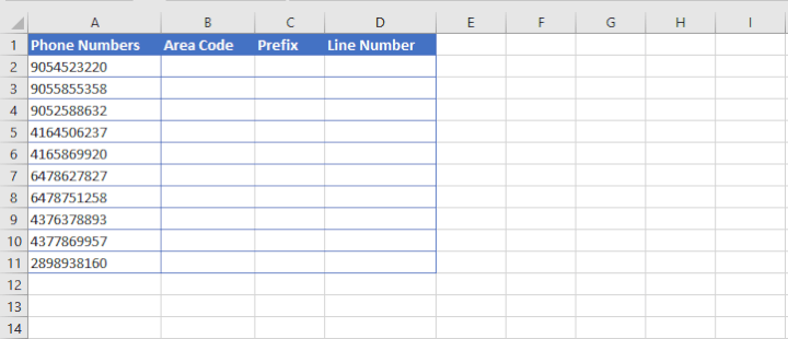
For example, the following dataset contains telephone numbers which we would like to split into three separate columns as follows:

• The area code, consisting of the first three numbers 
• The prefix, consisting of the next three numbers 
• The line number, consisting of the final four numbers 

Step 1

The LEFT function in Excel can be used to grab the first three numbers. The syntax of the LEFT function is:

=LEFT(text, [num_chars]

• Text is the text string to be split.
• Num_chars is the number of characters in text to return, starting with the leftmost character. If omitted, only the leftmost character is returned.

=LEFT(A2,3)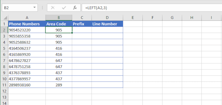

With the above formula, Excel extracts the three leftmost characters from the string in cell A2.

Step 2

Then we can use the MID function to get the next three numbers. This is an easy plug-and-play since the starting position and the length of the desired substring are known.

=MID(A2,4,3)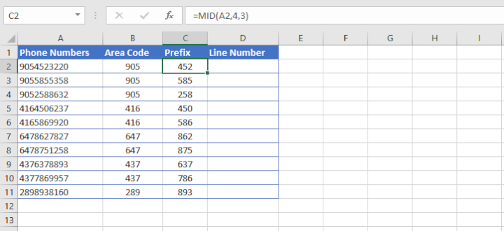

In the above formula, we are asking Excel to extract three characters from the string in cell A2, starting with the fourth character from the left.

Step 3

Finally, we use the RIGHT function to extract the last four numbers. The syntax of the RIGHT function is:

=RIGHT(text, [num_chars])

• Text is the text string to be split.
• Num_chars is the number of characters in text to return, starting with the rightmost character. If omitted, only the rightmost character is returned.

=RIGHT(A2,4)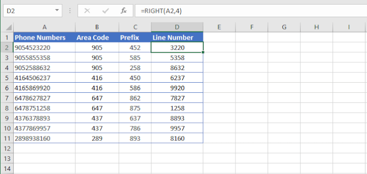

Now we have successfully split the text in one cell into three cells using a formula. This is a great solution for text strings that are of fixed length. Learn how to use the RIGHT function in Excel here.

Splitting text of variable length

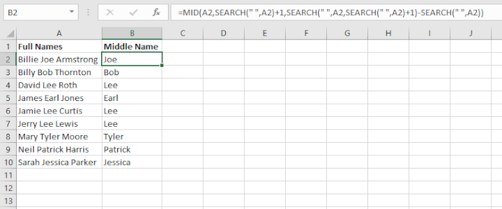
How about trying to get the middle names from the following list? 

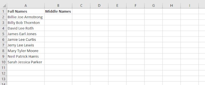
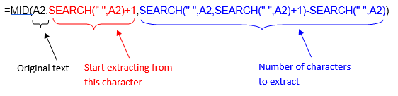
Obviously, we can’t use the basic MID syntax, since the names are all different lengths. The one thing they do have in common is that there is a space character before and after each middle name. Let’s work that into our formula.

Step 1

The first step is simple. We need to find the position number of the first space character. We can use the standard SEARCH function.

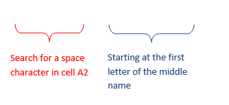
=SEARCH(“ ”,A2)

The result is 7, meaning the first space character is in the seventh position of the text string, so we now know that the middle name starts with character number 8. 

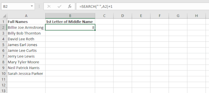
This information will later be used as the start_num argument of the MID function.

But now how do we know where the middle name ends? That is, what will we use to determine the num_chars? We need to identify the position of the second space character in the original text, which requires a little bit of Excel function gymnastics.  

We can think about it this way - assuming that we start looking from the 8th character in the string, where would the next space character be?

Step 2

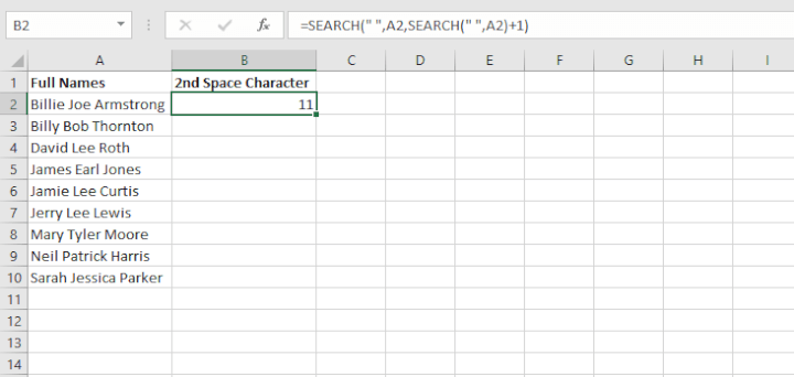
We already know that SEARCH(“ ”,A2)+1 tells Excel where the middle name starts, so let’s use that same location to start searching for the next space character.

 

SEARCH(“ ”,A2, SEARCH(“ ”,A2)+1

This formula will return the position number of the second space character from the original text string.

Step 3

The only thing left to do now is to use the MID function to look at the text in cell A2 (text argument), and starting with the eighth character (start_num argument), extract three characters (num_chars argument).

SEARCH(" ",A2,SEARCH(" ",A2)+1)-SEARCH(" ",A2))

The final SEARCH(“ ”,A2) element ensures that the number 11 will be subtracted from the position number of the first space character. 

We now pull all these elements together as arguments of the MID function.

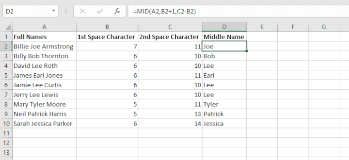
This formula gets the job done, but you might not be quite comfortable working with so many nested functions just yet. If that’s true, then you might find it easier to create columns for rough work, and use the result of those formulas to get the same results.

After Step 1 above, just determine the location of each space character step by step, and use those cell references as the arguments for the MID function.

MID function not working

If you can’t seem to get your MID function to return the result you expected, check out the following troubleshooting tips:

1. How to get a numeric output with MID 

As discussed before, MID returns values in Text format. If you want the return value stored in Number format instead (maybe you want to do a mathematical calculation on these numbers later), you can use the VALUE function to convert the output to their numeric values. 

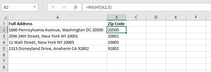
For example, we can extract the last five characters from a text string to get the zip codes from an address. However, notice that the numbers are aligned to the left of the cell. This indicates that these values are stored as text instead of numbers.

We can wrap the VALUE function around our formula to return a Number format. 

=VALUE(RIGHT(A2,5)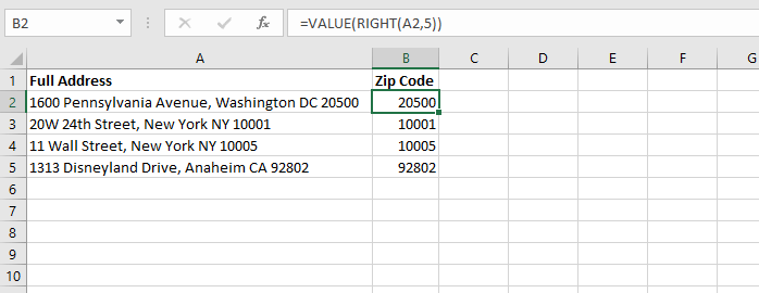

Notice that the numbers are now aligned to the right, indicating that they are stored in Number format.

1. Incorrect number of characters returned

There may be a couple of reasons for this. 

Extra spaces. If you know how many characters make up your desired output, but your MID formula only returns some of the characters, maybe there are extra spaces in your original text. 

The formulas in Column B were created to extract the seven-character postal codes, but cell B2 is missing the last number. This is because there is an extra space between “A” and “0”. This sometimes happens when data is entered manually, and can easily be missed. 

We can fix this by combining MID with TRIM. The TRIM function in Excel is designed to remove all spaces from a text string except for one space between words.

=MID(TRIM(A2),5,7)

Quick note on combining functions: If you’re just learning how to nest (combine) functions, here’s a golden tip: whatever action you want Excel to perform first should be in the inner parentheses. This is because since the result of those calculations will be needed for the other function(s), Excel wants to store that information in its memory for the subsequent actions.

That’s why for the situation above, we trimmed the full address first, then extracted the seven characters we want. If we did it the other way around, TRIM(MID(A2,5,7)), the extra spacing would still be there. 

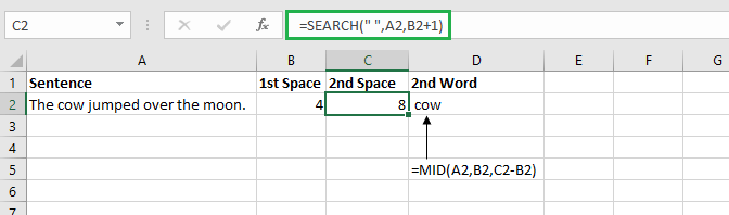
Working with delimiters. One reason may be that if you are using MID in combination with a function like FIND or SEARCH to establish delimiters, you may need to add or subtract one to the position number for your start or stop point.

For instance, if you wanted to grab the second word from the cell below, you would search for the first and second space characters. Remember to add 1 for the start_num argument for the second delimiter. Failing to do this could result in a return value that is the same position number as the first delimiter if both delimiters are the same. Adding a 1 tells Excel to start searching at the next character. 

3. Unexpected result when working with dates 

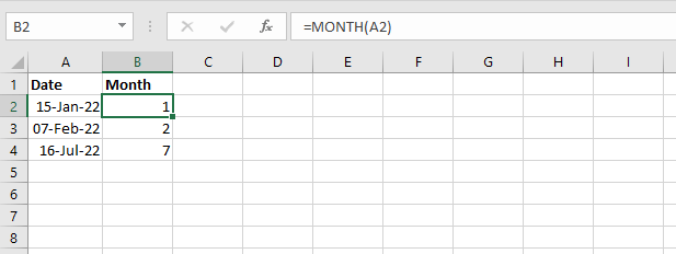
Since MID is a text function, it doesn’t handle numerical values well on its own. In the example below, we want to extract the month from the dates in Column A.

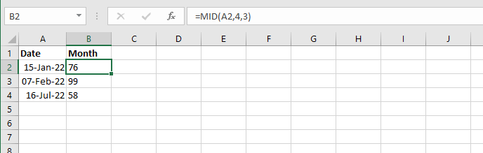
In this case, MID just isn’t the best tool for the job. Dates are really just numbers displayed in a way that makes sense to us. But for Excel, the date displayed as “15-Jan-22” is stored as a number string. So when we ask Excel to use the MID function to pull characters from that string, Excel says, “OK” and returns a substring from the number string shown to us as “15-Jan-22”.

The MONTH function works better here. It will return the month number (1 - 12) in the output cell.

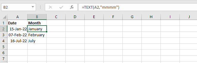
If you prefer, the month name can be returned by using the TEXT function instead.

MID vs. MIDB

If you’re interested in learning about MIDB, you’ll want to know that the only difference between MID and MIDB is that MID returns the number of characters in a text string, while MIDB returns the number of bytes used to represent the characters in a text string.

MIDB counts 2 bytes per character only when a double-byte character set (DBCS) language is set as the default language. The languages that support DBCS include Japanese, Chinese (Simplified), Chinese (Traditional), and Korean.

Otherwise, MIDB behaves the same as MID, counting 1 byte per character. For this reason, we have only discussed MID in this resource.

Next step

There are other ways to extract and split text in Excel. You just learned how the MID function works. Check out our resource library to learn other ways of managing data in Excel.

Level up your Excel skills

Become a certified Excel ninja with GoSkills bite-sized courses

Start free trial