The SUMIFS Excel Function

---

What is the SUMIFS Excel function?

The SUMIFS Excel function is used to add cells based on multiple user-defined criteria. It is a part of the IF family of Excel functions because it performs a certain action (in this case, it finds the sum of cells) only if the stated conditions have been met. These conditions may take the form of text, numeric values, or logical expressions.

The return value for the SUMIFS function is a single numeric output. Unlike the SUMIF function that accepts only one criterion, a total of 127 pairs of criteria may be submitted in a single SUMIFS formula, which translates to a maximum of 255 possible arguments.

---

---

How to use the SUMIFS function

The syntax of the SUMIFS function is:

=SUMIFS(sum_range, criteria_range1, criteria1,[criteria_range2], [criteria2]...)

Where:

• sum_range is the range of cells to be added.
• criteria_range1 is the first range of cells to be evaluated.
• criteria1 is the condition or criterion that cells in criteria_range1 must satisfy. 
• criteria_range2 is the second range of cells to be evaluated.
• criteria2 is the condition or criterion that cells in criteria_range2 must satisfy.

All arguments after criteria1 are optional. 

Basic application

Text criteria

The following example lists a database of subscribers and their outstanding balances. We can determine the total owed by premium tier subscribers in the United States by using the SUMIFS function. The two criteria are (1) “premium” and (2) “United States”.

The formula would be entered as follows:

=SUMIFS(F2:F18,B2:B18, “premium”, E2:E18, “United States”)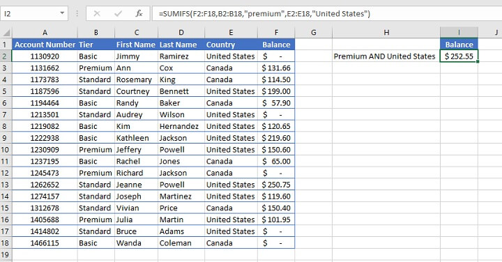

It is important to remember that the SUMIFS function uses AND logic to determine qualifying cells. This means that cells in the criteria ranges must satisfy all the stated conditions to be considered a match. 

If a row of data fails any of the stated criteria, that row will not be included in the results. Therefore, only the balances in rows 10 and 16 were included in the result above. Rows 3, 5, 8, 9, 10, 13, and 14 each met only one of the two criteria, and therefore did not qualify.

For cells that meet any of the stated criteria (OR logic) rather than all the stated criteria, the SUMIF function is more appropriate.

Cell reference criteria

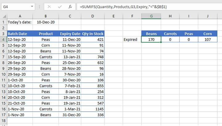
In the next example, inventory items are listed by batch date, expiry date, and the quantity in stock. Instead of using explicit text criteria within the SUMIFS formula itself, the criteria are listed in a separate location on the worksheet and referenced by the formula.

To determine the total number of each expired product, the SUMIFS formula would read:

=SUMIFS(D4:D17,B4:B17,G3, C4:C17, “<”&B1)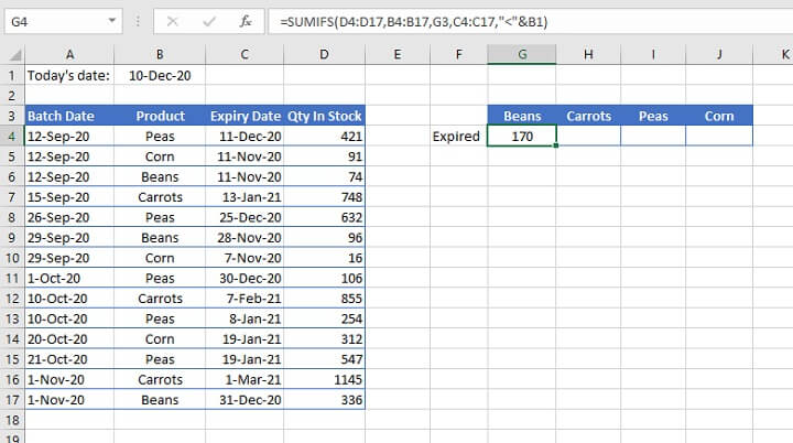

• In the above example, the third argument refers to the value in cell G3 (Beans). No double quotation marks are used because “G3” is not the literal value being extracted from the range.
• In the fifth argument, a cell reference is used to compare the dates in column C to the date in cell B1. Products that have expired would have a date earlier than (or less than) today’s date. Therefore the logical operator < is used and placed within double quotes. This format is followed by an ampersand (&) to concatenate, or join, the operator to the relevant cell reference.

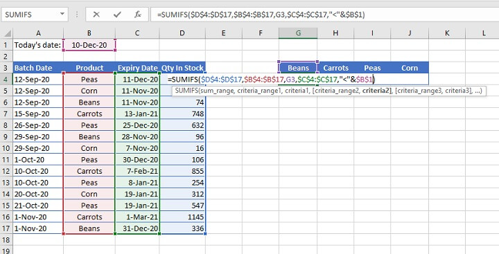
As a best practice and to reduce manual effort, cell ranges that should not change when copied to other cells may be entered as absolute references prior to being copied, as shown below.

Named ranges

Due to its use of multiple ranges, a SUMIFS formula can get quite unwieldy and difficult to read. It is, therefore, often beneficial to define a custom name for ranges that will be frequently used.

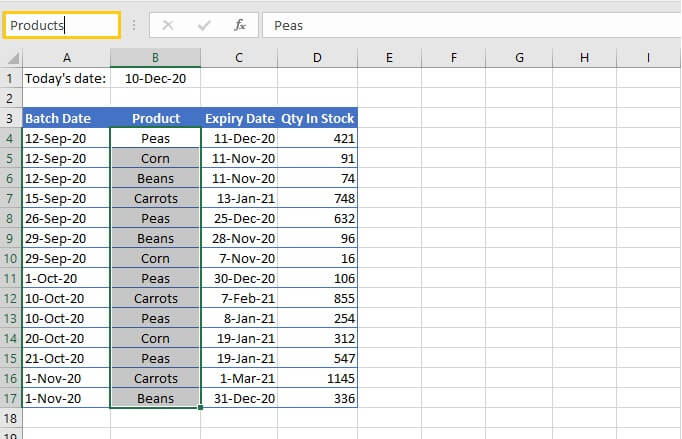
The steps to create a named range are as follows:

1. Highlight a range that will be used frequently.
2. Type a descriptive name in the Name Box (e.g., Products).
3. Press Enter.

A maximum of 255 characters are allowed in user-defined Excel names, and spaces are not permitted. Named ranges are valid on all sheets throughout the workbook.

Substituting named ranges where we previously had cell ranges results in a formula that is easier to read, and has the additional benefit of eliminating the need for absolute references. 

In the picture above, three named ranges (“Products”, “Expiry” and “Quantity”) have been used in the formula to replace the B4:B17, C4:C17 and D4:D17 references, respectively.

Criteria between two numeric values

For cells that are greater than one value and less than another value, the criteria_range would be repeated for the upper and lower limits of the criteria, as in the following example:

=SUMIFS(Quantity,Products,G3,Expiry,">=12/15/2020",Expiry,"<=12/31/2020")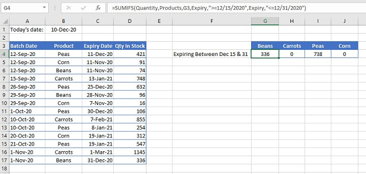

The formula calculates the total number of products that will expire on or after December 15 but no later than December 31. Note that explicit date references may be used as shown above. 

However, one disadvantage with this method is that if the file is shared to a computer with different regional settings, it may result in the SUMIFS formula searching for an invalid or incorrect date and returning inaccurate results. It is, therefore, a better practice to enter dates using the DATE function.

=SUMIFS(Quantity,Products,G3,Expiry,">="&DATE(2020,12,15),Expiry,"<="&DATE(2020,12,31))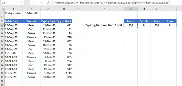

Note that in the above example:

• Only the logical operators are placed within double quotes.
• The ampersand symbol (&) is placed after the double quotes to concatenate, or join, the operator to the DATE function which follows.
• The DATE function follows a (year, month, day) syntax.

Other criteria 

The Excel SUMIFS function also supports wildcards for partial matches, and the <> (“is not equal to”) operator. 

An example of their application is shown below.

=SUMIFS(Balance,Tier,"<>premium",City,"*FL")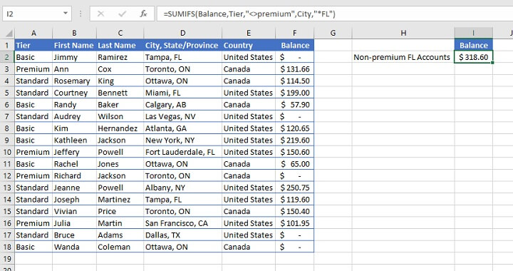

In the example above, named ranges have been used to identify the rows where the text value in the Tier range (A2:A18) is not equal to  “Premium”, and which have an unknown number of characters preceding the letters “FL” in the City (D2:D18) range. 

As a result, both rows 5 and 14 were isolated and their corresponding values in column D were added together.

Summary

The SUMIFS Excel function is a very powerful tool that you won’t be able to do without now that you’ve discovered it. 

Ready to learn more? Check out our library of Excel courses and other resources to level-up your Excel skills.

Start by trying our free Excel in an Hour course then level up with our Excel - Basic and Advanced course to learn more time-saving formulas and functions.

Learn Excel for free

Start learning formulas, functions, and time-saving hacks today with this free course!

Start free course