As an Excel user, you have probably heard of two of the most well-known features of Excel: the VLOOKUP function and Pivot Tables.
But if you have not used them much before, you may be wondering: When would you use VLOOKUP vs Pivot Tables? And what you should use them for?
In this article we will examine VLOOKUP, Pivot Tables and also Power Pivot, and when you should use each of them for best results.
Download your free practice file
Follow along with the steps in the article by downloading this practice file.
What is VLOOKUP?
VLOOKUP is a lookup and reference function in Excel.
It is commonly used in a worksheet to look up and pull data from another Excel table or worksheet.
For example, we have an Excel table named “Sales” which contains details of product sales for all months of the year.
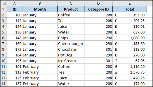
And another table named “Products” with product details.
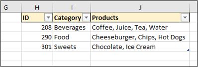
We would like to create a PivotTable showing the total sales by the different product categories.
However the “Sales” table does not have the details about the product categories. That information is stored in the “Products” table.
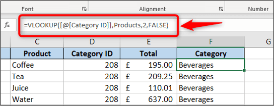
We can use the VLOOKUP function to bring the category information into the “sales” table.
How to use the VLOOKUP function
The VLOOKUP function has four arguments (information it needs).
They are the lookup value, table array, col index num and range lookup.

Lookup Value is the value you are looking for. This is the category ID in our example.
Table Array is the table we need to look up this information. This will be the “Products” table.
Col Index Num is the column number of the table containing the information to return. This will be the column containing the category, which is the second column. So we will use 2.
Range Lookup is the type of lookup you are performing. Are you looking in ranges? In our example we aren’t, because we are looking for a specific category ID.
The following formula is added to the “Sales” table in column F.
=VLOOKUP([@[Category ID]],Products,2,FALSE)
VLOOKUP is an extremely useful function in Excel that can be used in many other clever ways such as to compare lists or test values.
In addition to VLOOKUP, the INDEX and MATCH formula is also very useful to look up data from other Excel tables.
What is a Pivot Table?
A Pivot Table is a reporting tool in Excel that summarises data and performs an aggregation on values.
For example, to show total sales by month or number of orders for each product.
It is very powerful and makes generating reports quick and simple.
How to create a Pivot Table
With the category column now in the “Sales” table, we can create the Pivot Table to show the total sales for each product category.
Click in the “Sales” table, then click Insert > PivotTable.
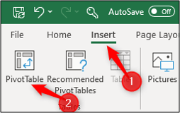
The “Sales” table is picked up as the data source to be used. And the default option is to insert the Pivot Table on a new worksheet.
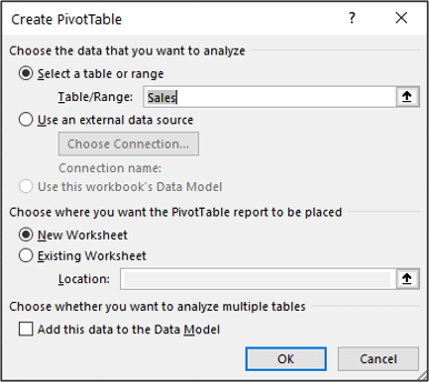
The new worksheet is inserted and the PivotTable placed on it. A field list is shown on the right with all the columns from the “Sales” table.
Click and Drag the “Category” field into the Rows area of the Pivot Table, and the “Total” field into the Values area.
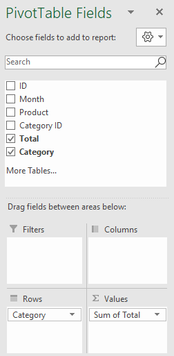
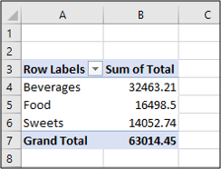
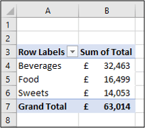
The Pivot Table shows the total sales for each product category.
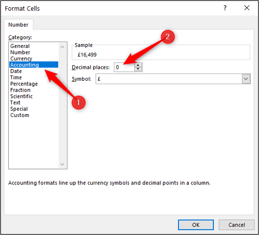
To format the values correctly. Right-click a Pivot Table value and click Number Format.
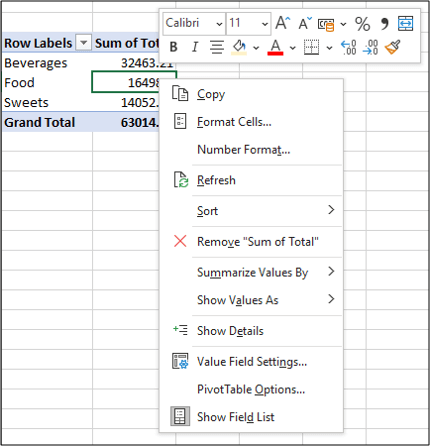
Choose the formatting you would like to use. In this example, I have selected Accounting with 0 decimal places.
The Pivot Table is now correctly formatted.
Pivot Tables are a powerful Excel tool. Check out some advanced Pivot Table techniques.
What is Power Pivot?
Power Pivot is also referred to as the data model in Excel.
In simple terms, it enables us to create a Pivot Table from multiple tables, which it refers to as the data model.
Power Pivot is an advanced feature including its own formula language called DAX. You can learn more about it in this comprehensive guide to Power Pivot.
Keeping things simple however, it can also be used as an alternative to VLOOKUP.
Instead of using a lookup formula to consolidate data from multiple tables into one, you can keep them in their own tables and use Power Pivot to relate them.
You can then create a Pivot Table from all the related tables (the data model).
Load tables into Power Pivot
First, you need to load the tables into the data model.
Click in the “Sales” table and click Data > From Table/Range.

This will open the Power Query Editor window.
Power Query is a tool to make powerful transformations to your data to make it ready for analysis. It is great for preparing data for Power Pivot.
This data is clean and requires no transformations, so it can be loaded straight into the data model.
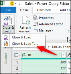
Click Home > Close & Load > Close & Load To.
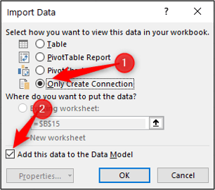
Select the option to Only create connection and check the box to Add this data to the Data Model.
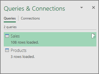
The table is loaded into the model. This will be shown in the Queries and Connections window.
Repeat these steps for the “Products” table.
Both tables are loaded into the data model and are visible in the Queries and Connections pane.
Create relationships between tables in the model
Now to create the relationship between the two tables, we need to open the Power Pivot window.
Click Data > Manage Data Model.

The Power Pivot for Excel window opens and takes you to the Data view.
It looks like an Excel workbook (but it’s not). The two tabs at the bottom of the screen are the two tables that were loaded into the data model.
Click the Diagram View button.

Click and drag from the “Category ID” field in “Sales” to the “ID” field in “Products”
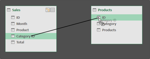
When you release your mouse, the relationship is created.
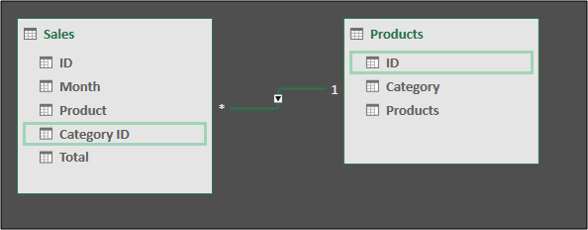
A line is drawn between the two tables with a 1 on the “Products” side and an infinity symbol on the “Sales” side.
This indicates a one-to-many relationship as a product can be sold many times.
Close the Power Pivot window.
Create a Pivot Table from a Power Pivot data model
Now that the tables are related, we can create a Pivot Table using both of them.
Click Insert > PivotTable.

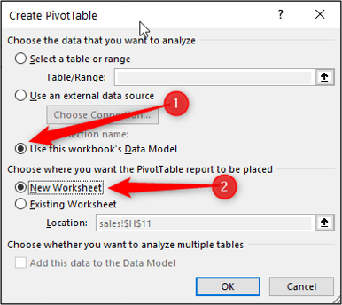
Ensure that the Use this workbook’s Data Model option is selected. Click New Worksheet as the location for the Pivot Table.
The Pivot Table is created and the Field List appears.
The Field List shows the two tables in the data model, and also the two tables on the worksheet.
We need to use the two in the data model. These are identified by the different icons next to their name.
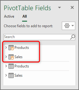
Drag the “Category” field from the “Products” table into Rows. And then drag the “Total” field from the “Sales” table into “Values”
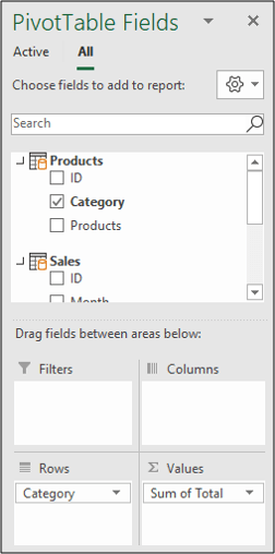
Format the values and we have the same Pivot Table results as before.

This time the tables were kept separate and related using the data model.
This is more efficient than writing several VLOOKUP functions to bring data from different tables into one. Especially when you are working with large data sets and multiple tables.
VLOOKUP to pull data from a Pivot Table
So VLOOKUP is commonly used to consolidate data ready for a Pivot Table, but can it be used to return values from a Pivot Table.
Yes. Below is an example of a VLOOKUP function being used to return the total sales of food from the PivotTable we created.
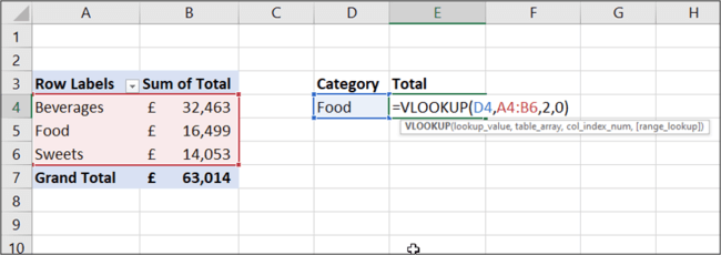
This returns the correct answer.
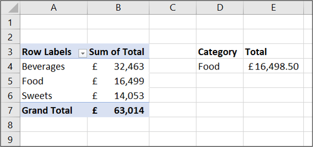
However, the VLOOKUP is using a reference to the cell range A4:B6. And although this works, if the PivotTable is changed the VLOOKUP will be broken.
It is not really pulling data from a Pivot Table, it is pulling it from the cell range.
VLOOKUP vs GETPIVOTDATA
So this could produce a problem. It depends what the Pivot Table will be used for and how.
Pivot Tables are a dynamic tool, but that VLOOKUP was not.
So a better approach may be to use the built-in Pivot Table lookup function called GETPIVOTDATA.
To use this function, type = and then click a cell in the Pivot Table.
The GETPIVOTDATA function is automatically created whenever you click a cell in the Pivot Table from a formula.

This example is using the Pivot Table created from the data model.
The GETPIVOTDATA function is looking up the value in the “Sum of Total” column and for the category of food.
So if the Pivot Table grew in size, GETPIVOTDATA would successfully retrieve the value. However the VLOOKUP would still look in range A4:B6 which would not be correct.
Wrap up
VLOOKUP and Pivot Tables are two features that complement each other. So it is more a case of how to use them together, rather than pitting VLOOKUP vs Pivot Table.
You normally receive tables from different systems and people. So VLOOKUP can help prepare the data for Pivot Tables to then perform analysis and reports from it.
Pro tip: XLOOKUP is the shinier, more-powerful, easier-to-use upgrade to VLOOKUP.
Power Pivot offers an alternative approach to this by relating the different tables from which to create Pivot Tables.
Download your free practice file
Follow along with the steps in the article by downloading this practice file.
Learn more with GoSkills
Want to learn more about Excel? Check out GoSkills comprehensive online Excel courses.
The Basic and Advanced Excel course can help you go from novice to Excel ninja, while the Pivot Tables and Power Pivot courses help you advance further into Excel mastery. Each course starts from the basics, so you have a solid foundation to build your knowledge and skills.
Sign up for a 7 day free trial today to try out all courses on GoSkills, including our award-winning Excel courses.
Ready to become a certified Excel ninja?
Start learning for free with GoSkills courses
Start free trial


