
After using Excel for many years, its power continues to surprise me on a constant basis. One of the best formulas and a personal favorite that’s included in almost every Excel 101 article is VLOOKUP. But what if I told you there are two other formulas, when used together, that make the VLOOKUP pretty much obsolete. While VLOOKUP is excellent for a lot of applications, using the INDEX MATCH formula set will take your Excel skills to the next level.
Step up your Excel game
Download our print-ready shortcut cheatsheet for Excel.
VLOOKUP basics
Before we can truly appreciate the INDEX MATCH formula, let’s take a look at what has made VLOOKUP such a favorite tool. This formula is used to lookup up and retrieve data in a table based on search criteria.
The V in its name conveniently stands for vertical, which means the formula will search for the criteria vertically in the first column of the data. (Note: Excel has another function, the HLOOKUP, that does the same thing, just horizontally.)
The VLOOKUP formula works if your data is organized vertically and the search column is the left-most column. Let’s look at an example of what goes into a VLOOKUP formula.
=VLOOKUP (lookup_value, table_array, col_index_num, [range_lookup])
- lookup_value is the value to search for in the left-most column of the table.
- table_array is the range of cells that contains the data being searched.
- col_index_num is the column number in the table relative to the first column in the table.
- [range_lookup] specifies if an exact match or the closest match is required. Excel uses the exact match by default if not specified.
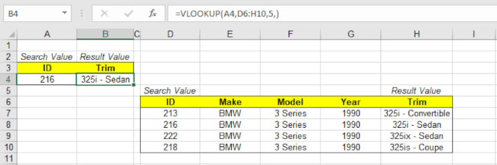 In the example above the formula is: =VLOOKUP(A4,D6:H10,5)
The lookup_value of “216” in cell A4 is returning the result of “325i - Sedan” which is the 5th column of the D6:H10 table for the corresponding row.
VLOOKUP drawbacks
Unfortunately, dealing with data isn't always straightforward. Sometimes layout changes or additional columns are added and updating all your VLOOKUPs can be time-consuming depending on how many you have. Let’s look at just a few of the limitations you face using VLOOKUP.
Inserting new rows or columns
The VLOOKUP formula uses what's known as a static column reference. This is a fancy way of saying the specs of your formula do not update when you make table changes. Taking the same example from above, if we added a column for Horsepower between the Year and Trim columns, the VLOOKUP formula would now pull in the results from the horsepower column instead of the Trim column.
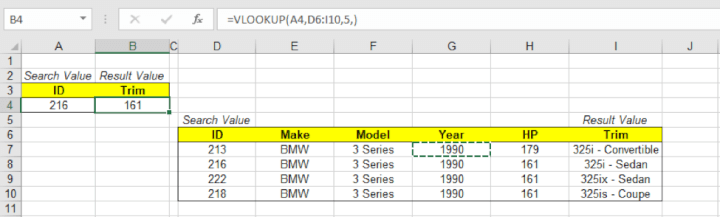 Not a big deal with just a few formulas, but when updating a large amount you would risk your data being inaccurate.
Data organization
When it comes to the VLOOKUP formula, there are two sore spots related to data organization. First, your data has to be set up with the search column in the left-most column of your table. Second, if you use the approximate match for the range_lookup, the data needs to be organized in ascending order. While these two aspects seem minor when applied to tables with a large amount of data they can cause a headache.
Lack of flexibility
The VLOOKUP formula works in a particular way to search for data. If you need to search horizontally, there’s an entirely different formula for that, the HLOOKUP. While these are both useful, if you have to learn multiple formulas, it's better to learn the ones that provide the most benefit overall.
Counting columns
Since VLOOKUP references are static, you typically have to count the number of columns in your table to get to the results you’re looking for. This is the adult version of counting on your fingers. Let's face it, we are using these formulas to make quick work of searching through data and that time should be spent analyzing the results and not counting columns.
Why INDEX MATCH?
Where the VLOOKUP is lacking, INDEX MATCH picks up the slack. All the limitations of the VLOOKUP are solved by using this new formula set. So what exactly is the INDEX MATCH formula and how does it make searching through data so much easier? First, let’s take a look at the different pieces that make up the formula.
Nestle in with nested formulas
When learning Excel, most people start with simple, single function formulas. This is another part of what has made VLOOKUP so popular is its simplicity. But once the training wheels come off, you start using different formulas together to create more complex functions using the concept of nesting.
Nesting means using multiple stand-alone formulas in a single formula. Most of the time nesting is used for conditional formatting like multiple IF formulas. But the nesting possibilities don't stop there. The INDEX MATCH formula is the common term for nesting a MATCH formula in an INDEX formula, to search just like the VLOOKUP. Let’s take a more in-depth look at the two formulas separately to ease the confusion.
INDEX
The INDEX function returns a value in a table based on a set of coordinates for the column and row. Think of this like global coordinates of longitude and latitude where the longitude coordinate is the column, and the latitude coordinate is the row. The first row in the table is row 1, and the first column in the table is column 1. The following are the components of the INDEX formula:
=INDEX(reference, [row], [column])
- reference is the table of data. This can be a single range or the entire data set.
- [row] is the row coordinate in the reference.
- [column] is the column coordinate in the reference.
- Note: Variables to the formula with [brackets] are optional. In this example, if there is neither row nor column specified, the INDEX formula would return the entire reference as a new table.
Using the following example, here’s how it works.
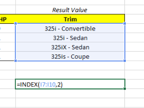 In the example above the formula is: =INDEX(I7:I10,2)
- The reference is the range I7:I10.
- The [row] value will return the 2nd row in the table.
No column coordinate was selected as the there is only one column to choose from. Had there been two columns, the INDEX formula would have returned all values for all columns for the specified row.
Now that the INDEX is set let’s turn to the MATCH function to determine how we determine the row value.
MATCH
The match formula searches for a given value in a range of cells and then returns the relative position in that range in the form of a coordinate. Basically, MATCH is a less refined version of a VLOOKUP or HLOOKUP that only returns the location information and not the actual data. The following are the components of the MATCH formula:
=MATCH(lookup_value, lookup_array, [match_type])
- lookup_value is the value searched for in the lookup_array.
- lookup_array is the range of cells to search for the lookup_value.
- [match_type] is a qualifier. 1 is searches for a value greater than the lookup_value, 0 returns the exact match, and -1 returns the value less than the lookup_value.
- Note: match_type defaults to exact match if excluded.
Continuing with our example, here’s what MATCH returns.
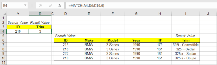 In the example above the formula is: =MATCH(A4,D6:D10,0)
The lookup_value of “216” in cell A4 returns the exact match (denoted by the zero in the formula) of the lookup array D6:D10.
We see that the Trim value is now 3, which is the location of 216 in the array D6:D10.
Putting it all together
So INDEX is used to return a value based upon coordinates, which are basically variables. The MATCH formula returns the variable based upon where the search criterion is in its range. This then fills the coordinate(s) for INDEX and voila!
Now when you add a column or manipulate your data, you won’t have to update references that were Excel version of a stick in the mud. To solidify your understanding here is a view of the formula and the value returned.
 Formula view of the INDEX MATCH
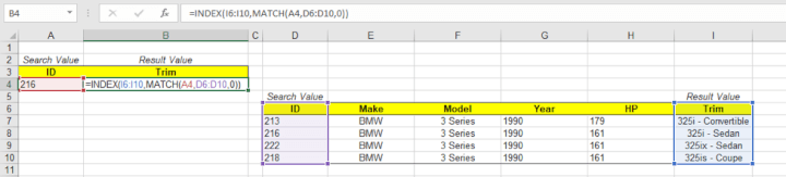
In the example above the formula is: =INDEX(I6:I10,MATCH(A4,D6:D10,0))
The reference is I6:I10
The [row] is MATCH(A4,D6:D10,0) which returns “3” since the lookup_value is the 3rd value in the lookup_array.
There are two different ranges you will have to specify, one for MATCH and one for INDEX. The first range will be the result values you want to return. The second range will be your search column.
The two ranges must contain the same number of rows or columns to work correctly depending on if you are searching vertically or horizontally. Otherwise, the formula will return an error message.
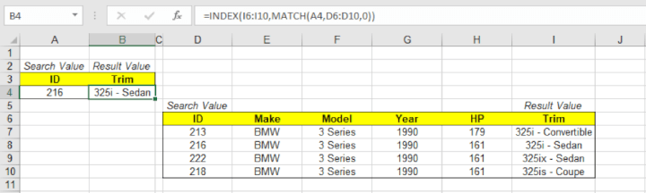 The regular view of the INDEX MATCH
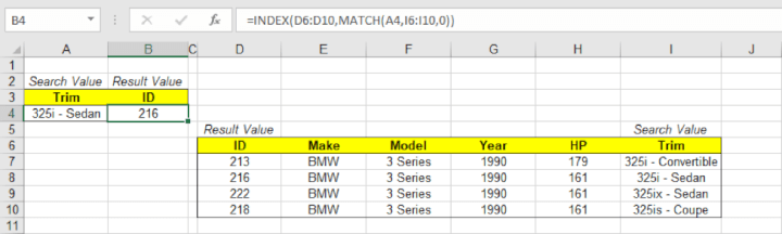
So say you want to find the ID, but all you know is the Trim? Ten minutes ago you would have had to reorganize your table for a VLOOKUP to work. But now that you’re older and wiser you know INDEX MATCH can handle this no problem.
INDEX MATCH is unmatched
Hopefully, after reading this, you now see why the INDEX MATCH is far superior to the VLOOKUP. Not only can you change your data without updating references, but you also don't have to worry about rearranging your data to fit the constraints of a VLOOKUP. If you are geeking out about this formula and want to try your hand at it, feel free to download the attached Excel workbook for a data set to test your skills. Once you get your bearings using INDEX MATCH, you’ll wonder why you ever used a VLOOKUP.