9 minute read

What is INDEX MATCH in Excel?

Claudia Buckley

INDEX MATCH is a clever way to do a two-way lookup in Excel, and it can be used as a workaround for the limitations of VLOOKUP.

For example, VLOOKUP only works when the lookup value is in the first column of the lookup array. It also cannot accept lists sorted in descending order, or return a value that is to the left of the lookup value.

If you use VLOOKUP regularly, you may have come across these problems and probably just decided to live with them. Learning how to use INDEX MATCH is a great workaround.

INDEX MATCH is made up of two functions. The MATCH function is used to figure out where the lookup value is located in a range of cells. The INDEX function then returns the value or cell reference from within a table or range.

The MATCH and INDEX functions are combined to do the job that VLOOKUP cannot do. This includes looking up values that are to the left of the lookup value, accepting approximate matches when the list is sorted in descending order, and even returning values that match multiple criteria. .

Let’s break down each of these functions step by step.

How to use the MATCH function

The MATCH function is used to determine the position number of a known value within a range of cells. The MATCH function in Excel has three possible arguments, with the following syntax:

=MATCH(lookup_value,lookup_array,[match_type])

Lookup_value is the known value that you will be using to conduct a lookup, or search. This can be a value or cell reference.
Lookup_array is the range of cells where the lookup value will be found.
Match_type is a setting that tells Excel whether you will accept a near-match if the lookup_value is not found in the lookup array.

Array Type	MATCH formula match_type
0	Exact match
1	Approximate match, to closest value smaller than lookup value
-1	Approximate match, to closest value larger than lookup value

For instance, if we wanted to know the position number of the word “matte” within the range B2 to B9 below.

=MATCH("matte",B2:B9,0)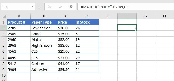

MATCH example

Note that in the example above, the value “matte” was typed directly into the formula between double quotation marks. If the lookup value is a cell reference, no double quotes are used.

Note also that the MATCH function is not case-sensitive.

How to use the INDEX function

The Excel INDEX function returns a value or cell reference from within a table or range. The INDEX function has two formats - the array format and the reference format. The array format is used when we want to return the value that is found in the result cell. The reference format is used when we want Excel to return the cell reference of the result cell (e.g. D17). We’ll focus on the array format, since this is the format you’ll need to learn for the INDEX/MATCH combo.

The syntax of the INDEX array function is

=INDEX(array, row_num, [column_num])

Array refers to the range or array containing the data to be indexed. This argument is required.
Row_num is the row number where the cell containing the return value is to be found. Row_num can be omitted if the array consists of only one row. If row_num is omitted, column_num is required.
Column_num is the column number where the cell containing the return value is to be found. Column_num is optional, but is required if row_num is omitted.

In the spreadsheet below, we want to display the value which is in the third row, second column of the array by using the INDEX function.

=INDEX(A2:D9,3,2)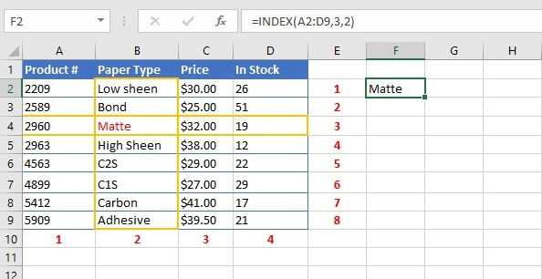

INDEX example

The third item in column 2 is identified as the value “Matte” and returned as the output in cell F2.

Download your free INDEX MATCH practice file!

Get the Excel file to follow along.

Combining the INDEX and MATCH functions

As mentioned before, the INDEX and MATCH formulas, when nested, can perform a lookup that accomplishes what the VLOOKUP does and more. Nesting a formula means using one entire formula as an argument of another function.

We can apply that to our simple query which extracts values from a dataset using the Product Number as an input or lookup value.

INDEX MATCH example

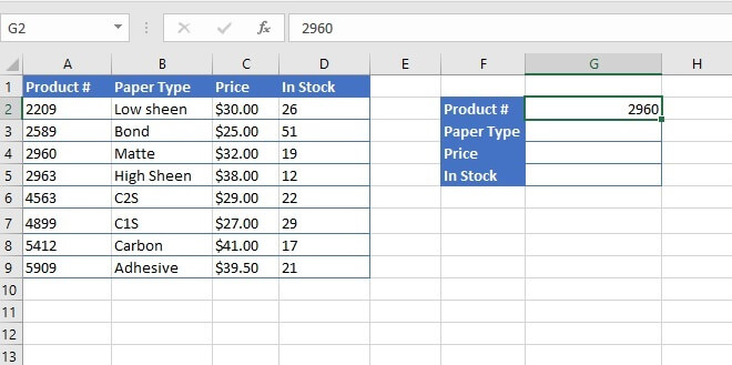
We will use MATCH to determine where in the list the product number falls (position number), and we will use INDEX to return the values from the corresponding columns (Paper Type, Price, or In Stock,) by their column numbers.

Shown separately, each function would read as follows:

=MATCH(G2, A2:A9,0)

This performs a search for the value in cell G2 within the A2 to A9 range, and requires an exact match. It returns the position number of that value.

=INDEX(A2:D9, row_num, 2)

This returns the value from the array A2 to D9 which intersects the row number found in the MATCH formula, and column number 2 (Paper Type). The MATCH formula will be used as the row_num argument.

=INDEX(A2:D9,MATCH(G2,A2:A9,0),2)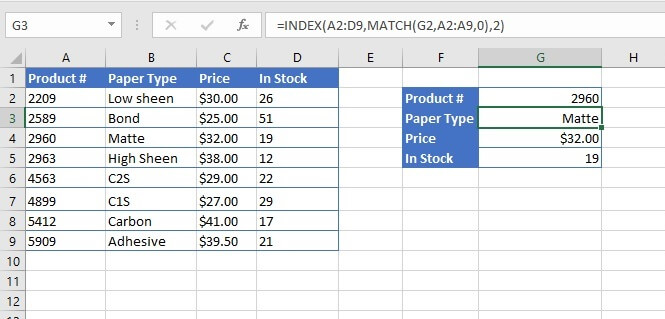

INDEX MATCH example 2 The formula in G4 and G5 are identical, except for the last argument, which are 3 and 4 respectively, to represent each column number.

To be fair, this does seem quite complicated when we consider that VLOOKUP already does this in a much more straightforward way, and with only four arguments. However, at the outset, we pointed out that VLOOKUP could not return a value that was located to the left of the lookup value.

If we change the known value so that the Paper Type is now our lookup_value, VLOOKUP returns a #NA (Value Not Available) error. Let’s see how INDEX MATCH handles this.

=INDEX(A2:D9, MATCH(G2, B2:B9,0),1)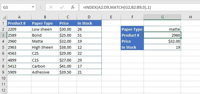

INDEX MATCH example 3

Lookups to the left or right are no problem for INDEX MATCH because the MATCH lookup_array stands on its own, and is not connected to the INDEX array.

In this way, INDEX MATCH can also be used as a substitute for HLOOKUP, which is the horizontal version of the VLOOKUP function.

Let's look at a more advanced application of the INDEX MATCH solution.

INDEX MATCH advanced example

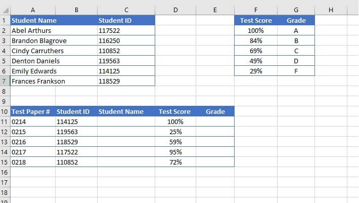INDEX MATCH example 4 Test-takers have entered their Student IDs on their test papers, which are then scored and the grades entered in column D. We want to look up the Student ID in the array A2 to C7, but VLOOKUP is unable to do so. The student names are displayed to the left of the ID numbers because the list is arranged alphabetically. That is our first problem.

We also want to assign a letter grade based on each student’s test score. The test score chart (F2 to G6) is sorted in descending order, which is another thing VLOOKUP cannot handle.

The MATCH function will be used to determine the row number of the INDEX function.

=MATCH(B11,$C$2:$C$7,0)

(The range C2 to C7 will be copied, so we can use $ to make the references fixed. Learn more about Absolute and Mixed References.)

We used match type 0 to ensure that only an exact match will be returned.

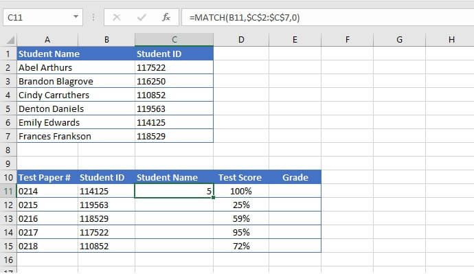INDEX MATCH example 5 The MATCH function located Student ID 114125 in position 5 of the lookup array.

Now we just need to link that to the corresponding student name.

=INDEX($A$2:$C$7,MATCH(B11,$C$2:$C$7,0),1)

(The range A2 to C7 will be copied, so we can use $ to make the references fixed. Learn more about Absolute and Mixed References.)

The MATCH formula has been inserted, or nested, within the INDEX function as a way to find out what row is to be returned in each instance. The first column of the array contains the value we want returned, so the last argument of the INDEX function (column_num), is 1.

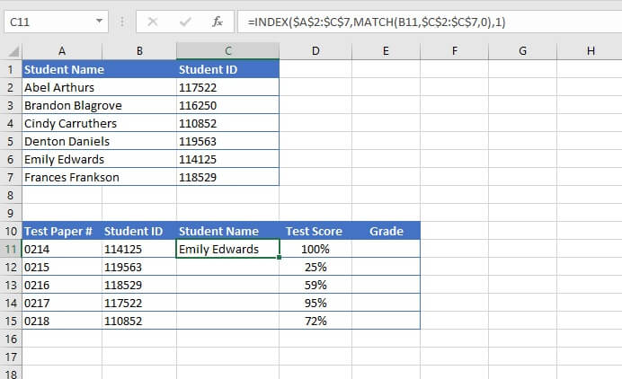INDEX MATCH example 6 This formula can now be copied to the remaining rows in column C.

Determining the letter grade for each student will follow a similar pattern, with one exception. Since the grading chart only lists five values, students’ test scores may not be an exact match, therefore the match_type in the MATCH formula must be adjusted to accept an approximate match.

INDEX MATCH example 7

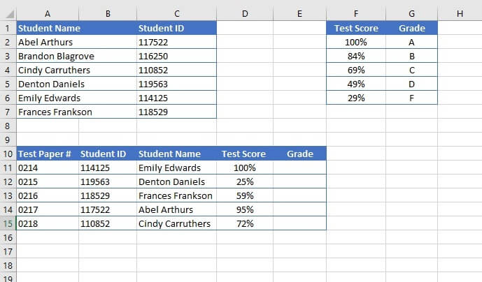
Our MATCH and INDEX formulas would read

MATCH(D11,$F$2:$F$6,-1)
INDEX($F$2:$G$6,nested MATCH formula,2)

When nested, the complete formula would be:

=INDEX($F$2:$G$6,MATCH(D11,$F$2:$F$6,-1),2)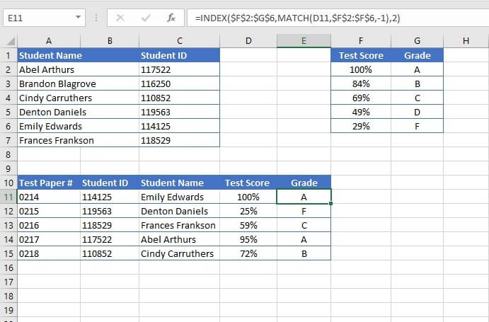

INDEX MATCH example 8

So although VLOOKUP was made to simplify the common task of finding items in a table, we can’t discard INDEX MATCH for more advanced tasks.

Here’s something you might want to know - Excel has rolled out XLOOKUP as the fix for the above complaints about VLOOKUP’s limitations. The drawback is that it’s only available in Excel 2021, Excel for the Web, or with a subscription to Microsoft 365, so if you have an older version, you’ll definitely want to understand and master INDEX MATCH.