How to Count Unique Values in Excel with the UNIQUE Function

If you’ve ever wanted to count the number of unique values in an Excel range, you’ll know that there was really no easy way to do it. You would either have to create a pivot table or a complex array formula from a series of nested functions. 

This isn’t welcome news for beginners, or even for some intermediate Excel users, so it’s great to know that with Microsoft 365 there is now a dynamic array function in Excel that takes care of that. To help you count unique values, Excel offers the UNIQUE function.

The UNIQUE function in Excel can either count the number of distinct values in an array, or it can count the number of values appearing exactly once. UNIQUE accepts up to three arguments and the syntax is as follows:

=UNIQUE(array, [by_col], [exactly_once])

• Array is the range or array to be evaluated.
• By_col (optional argument) tells Excel whether the data in the array is displayed row-by-row or column-by-column. If this argument is omitted, Excel assumes the data is vertical (i.e., across several rows). If not, enter TRUE (jump to an example for more details).
• Exactly_once (optional argument) is like choosing a “distinct” versus “unique” setting (see below). The default setting is distinct. To display only unique values, enter TRUE (jump to an example for more details).

---

---

Distinct vs unique values

Extracting a list of distinct values means that each value from the original list is shown but without their duplications.

Unique values, on the other hand, are values that appear only once in the original list.

The option to choose between distinct and unique is in the third argument of the UNIQUE function. If the third argument is omitted, then “distinct” is assumed.

Required argument and defaults

The basic UNIQUE function has only one argument. To extract a list of each item listed in the range A2 to A8, we enter:

=UNIQUE(A2:A8)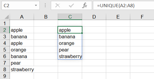

There is no need to enter the optional arguments because:

1. The A2 to A8 range is vertical (row-by-row), which is the default.
2. We want a list of all the values that appear in the original list, but without their duplications.

Excel returns a “spilled” list, displaying all of them in the same format (vertically) as the original list. The values “apple” and “banana” are duplicated. Hence, they are only returned once in the output list. 

If there are not enough empty cells to display all the spilled values, Excel will return a #SPILL! error.

Horizontal ranges

If your array is a horizontal range (i.e., displayed across several columns), you should enter TRUE as the second argument in the UNIQUE function. To extract distinct values from the range A2 to G2 below, we use the following formula:

=UNIQUE(A2:G2,TRUE)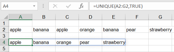

Entering TRUE for the second argument [by_col] tells Excel that the list is horizontal. This may seem counter-intuitive, but is in fact correct, because the values are found in separate columns (A to G, in this case).

Excel returns a “spilled” list, displaying them in the same format (horizontally) as the original list. The values “apple” and “banana” are duplicated. Hence, they are only returned once in the output list.

If there are not enough empty cells to display all the spilled values, Excel will return a #SPILL! error.

No third argument was entered in the above example because we want a list of all the distinct values that appear in the original list. This is the default setting of the UNIQUE function.

Show values that only appear once

The third argument of the UNIQUE function is exactly_once, and it’s optional. If TRUE is entered, Excel extracts only values that appear exactly once within the array. 

To get this result in the example below, the formula entered is:

=UNIQUE(A2:A8,,TRUE)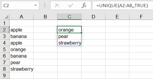

In this interpretation of “unique”, values that appear more than once are not returned in the results. Therefore “apple” and “banana” are removed from the results.

Note that in the above example there was no need to enter the second argument (by_col) since a vertical list is the default setting of the UNIQUE function. The second comma was entered as a placeholder.

Return numerical count of unique values

It may be that you are not interested in replicating the actual values from the original list but simply want to know how many of those values there are. Once you understand the UNIQUE function, it is quite simple to append it to the COUNTA function to get this answer.

Since COUNTA counts the number of cells in a range that are not empty, it doesn’t get any easier than combining it with the desired setting in the UNIQUE function.

To count the number of different cities listed from cells B2 to B18 below, we would enter:

=COUNTA(UNIQUE(B2:B18))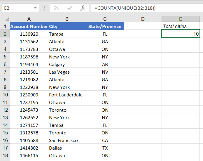

The result returned is that a total of 10 different cities are represented by the 17 accounts shown.

To determine the number of cities which have only one account holder, the third argument, exactly_once, is entered as TRUE.

=COUNTA(UNIQUE(B2:B18,,TRUE))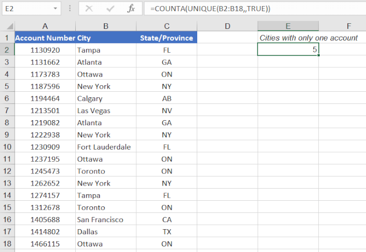

This principle also applies to the COUNT function to count unique numeric values.

Count unique values in Excel without the UNIQUE formula

If you’re not yet a Microsoft 365 subscriber, you may choose to use the UNIQUE function in Excel online. Since there is no backward compatibility for this function, it won’t work when opened with any older version of Excel.

So you may have to choose a more traditional method, like pivot tables.

Pivot tables are a great solution if you want a quick list or count of unique values in a dataset.

Steps to create a basic pivot table

1. Click anywhere within the dataset.
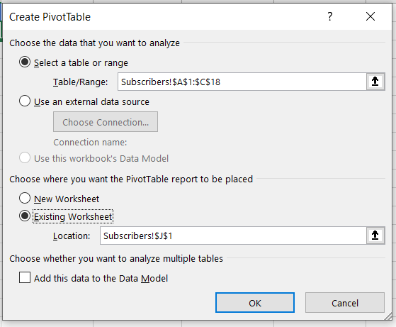
2. From the Ribbon, click Insert > PivotTable.
3. With the entire range selected, choose New or Existing Worksheet as the location of your pivot table.

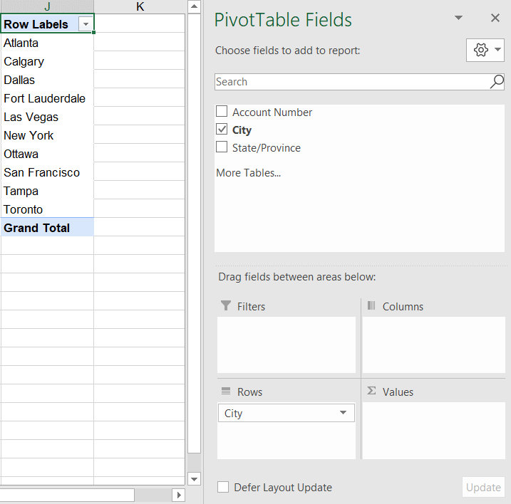
4. After selecting OK, a PivotTable Fields panel will appear, allowing the selection of desired summary fields.
5. Select the field containing the relevant values, and drag to the “Rows” field. A list of each distinct value will be displayed on the worksheet in the specified location.
   
   

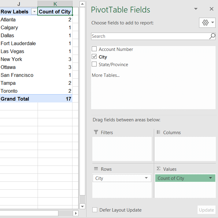
6. To get the total number of occurrences of each value, drag and drop the "City" field name to the Sum Values (∑ VALUES) area.
   
   

7. To display only the values which appear exactly once within the dataset, click the Filter arrow on the pivot table, select Value Filters > Equals > enter 1.
   
   

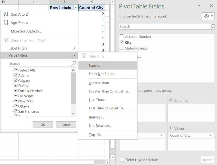
8. A list with values appearing exactly once in the original dataset is displayed.
   
   

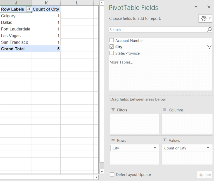
There are five cities appearing only once in the source dataset.

Learn more

These are just two ways we can extract unique values from a dataset. If you'd like to learn more essential Excel functions, formulas, and techniques - we can help!

Sign up for our Excel - Basic and Advanced course today!

Ready to become a certified Excel ninja?

Start learning for free with GoSkills courses

Start free trial