10 Most Common Excel Errors (and How to Fix Them)

An error can be defined as a mistake. More broadly, errors are actions that should not have happened or which lead to undesirable results. Excel has messages to alert us when we make certain types of errors. Seeing an Excel error message can be a bit frustrating, but it is much better than the other type of error – the silent one that goes undetected and returns inaccurate results.

Rather than getting irritated when we see an error message in Excel, consider it a welcome clue to identifying what went wrong so that you can go about fixing it. 

What to do when your Excel formula results in an error

First - don't panic! We've all gotten errors in our Excel functions at one time or another. Fortunately, Excel has some built-in tools to help you debug (or fix) the problem.

Step 1 - Check the error message

The most basic step is to look at the error message you're getting and use that to help you identify the problem. Of course, this means you need to be able to interpret what each error message means. That's where this little chart comes in handy.

Excel Errors - Quick Summary

Error	What it means	Why you're getting this message
######	-Can't display value	Your column is too narrow to display the output.
#CALC!	-Error in calculation	Excel doesn't know how to calculate the formula.
#DIV/0!	-Division by zero	Your formula is attempting to divide by zero.
#N/A	-Not available	The value you searched for is not available.
#NAME!	-Formula name error	Excel doesn't recognize the name of the function you entered.
#NULL!	-"Null" overlap	You requested the result of overlapping ranges (most likely a typo).
#NUM!	-Invalid number	The number is too large or too small to be displayed in Excel.
#REF!	-Invalid reference	A reference was deleted after creating the formula.
#SPILL!	-Spill area	The output area already contains a value.
#VALUE!	-Invalid value	An unexpected value was entered somewhere in the formula.

See below for detailed explanations.

Step 2 - Dig a little deeper

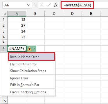
If you see a small green flag in the top left corner of your cell, you will likely also see a Trace Error button next to that cell. It means there is an error with your formula or the value inside that cell, and might even give you a bit more detail. When you hover over the icon or click the arrow next to the button, a list of options for dealing with the error will appear. You can select one of these to get into problem-solving mode.

Step 3 - Evaluate the formula in Excel

A more advanced option is to get Excel to trace what triggered the error, giving you a chance to correct it. For that, there is the Formula Auditing group of commands.

The fact is that if you understand what Excel is trying to tell you, you can usually figure this out on your own. Check out the following clues and suggestions, and you'll soon be saying, "Errors? What errors?"

How to fix Excel errors

Here is a detailed explanation of some of the most common errors in Excel, what they mean, and how to correct them.

1. ###### error

Whether you call them hashes, hashtags, pound signs, or number signs, seeing several of them in your Excel worksheet is usually a sign that Excel is trying to display a number, but the column is too narrow to show the number in full. This is an easy fix.

Possible solutions:

• The most common solution is to make the column wider. There are several ways to do this in Excel, but the quickest way is to double-click on the right column border at the top of the worksheet. This will automatically resize the column to the width of the widest value in that column.
• Alternatively, you can manually drag the column to a width that enables you to see the full value in that cell.
• If none of the above methods fixes your problem, then it’s time to step up your game. Maybe the value is saved in an incompatible number format.
• For example, do you have a negative value stored in date format? No matter how wide the column is, the ###### error will be displayed, as negative date values are considered invalid. To fix this, double-check the value or formula used to arrive at the result or change the number format from Date to another format, such as General.

2. #CALC! error

When Excel returns a #CALC! error, it may refer to any of several calculation problems related to array formulas. #CALC! may result from functions that are inherently dynamic or from formulas with an array syntax. For example, the FILTER function does not currently support empty arrays. If the condition defined within the include argument results in an empty array (i.e. does not exist), a #CALC! error will result.

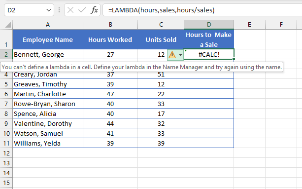
#CALC! may also be seen in the initial stages of defining/testing a LAMBDA function, and this means that the function has not yet been defined in the Name Manager.

Possible solutions:

• Include an if_empty argument in your FILTER function so that Excel knows what to do if there are no matching records for the specified filter criteria.
• Double-check the syntax rules for the function you are attempting to use. Check out our handy compendium of basic Excel formula how-to’s here.
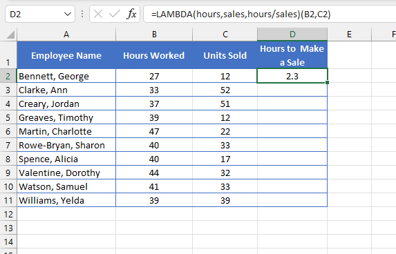
• If you are still in the testing stage of defining your LAMBDA, add a sample of the formula within parentheses to the end of your formula.

3. #DIV/0! error

At least the error message here is nice and clear, and it only means one thing - you are attempting to divide a number by zero. This operation is considered mathematically impossible, hence the division error message.

Sometimes the #DIV/0! error is unavoidable because there isn’t anything actually wrong with your formula. It could be that the divisor (denominator) in the formula references a cell that is currently empty or which returns a value of zero. Or, in the case of an AVERAGEIF formula, none of the cells within the range satisfy the criteria. In that case, it is not technically an error, but Excel cannot express the result because division by zero is undefined.

Possible solutions:

• The only way to truly fix this error is to remove the formula that is trying to divide by zero. This may mean:
  • correcting the divisor (denominator), or
  • deleting the formula
• If none of the above is a viable option, the IFERROR function is the best solution. IFERROR exists to catch or, more precisely, “cover up” errors so that they are not displayed in the output cell. IFERROR allows you to return an alternative result if the original formula results in an error.

4. #N/A error

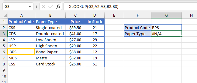
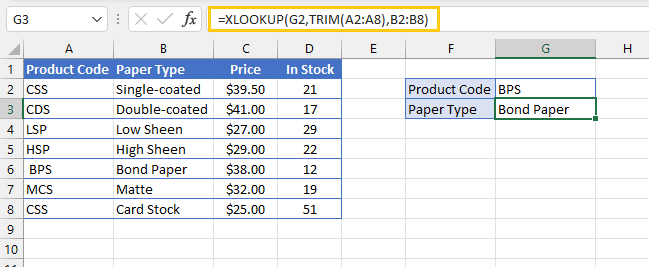
The #N/A error most often occurs when using a lookup function. This error indicates that the value you searched for is not available; that is, it wasn’t found in the source data. Sometimes it's as simple as a misplaced space character. For instance, in the following example, the product code in cell A6 has irregular spacing, so Excel has trouble finding the value entered in cell G2.

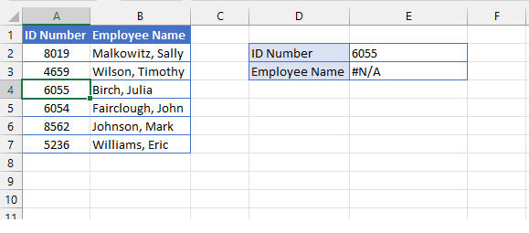
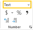
Occasionally, a #N/A error is the result of a formatting mismatch. In the example below, though the ID Number 6055 does exist in the source data, the value in cell A4 has been formatted as text, while the lookup value in cell E2 is formatted as a number. Excel concludes that they are not the same value. Therefore the lookup value was not found.

The N/A# error may also point to problems in the source data. For instance, in the following example, the product code in cell A6 has irregular spacing, so Excel has trouble finding the value entered in cell G2.

Possible solutions:

• Check the lookup value for typos.
• Select numeric values and change the format to Number.
• Use the TRIM function to remove extra spaces from the source data.

5. #NAME? error

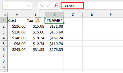
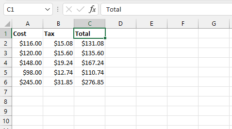
Whenever you see a #NAME? error in Excel, it means that Excel does not recognize the name of the function (built-in formula) you are trying to use. This is often the result of an error in spelling a function name or mistakenly placing an equal sign in front of the text.

Or you may have simply typed an equal sign in error. Since there is no Excel "TOTAL" function (see the SUM function if you're trying to find the total of a set of values), Excel returns a #NAME? error. 

Possible solutions:

• Correct the spelling of the function name if, indeed, you are attempting to use an Excel function.

 

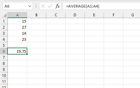
• Remove the equal sign if you are not trying to insert a function.

 

6. #NULL! error 

To understand the #NULL! error, think about a Venn Diagram. If the area where two circles overlap (or intersect) contains no values, it is said to be a “null” set. In Excel formulas, the space character works as an intersection operator.

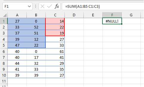
When Excel returns a #NULL! error, it means that you have (knowingly or unknowingly) asked for the result of two or more overlapping ranges, and Excel’s response is that it does not exist, because their paths do not cross or intersect. 

In the example below, the space between A1:B5 and B1:C3 refers to a valid intersection, i.e., B1:B3. Therefore the formula =SUM(A1:B5 B1:C3) returns the sum of the values in those cells.

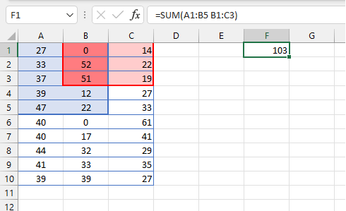
In reality, however, the most common reason for this is that you’ve typed a space between two cell references where you should have entered a comma to separate them, or a colon to separate the beginning of a range from its end. 

Possible solutions:

• To correct the #NULL! error, check the formula for incorrectly-placed spaces. Ranges should be separated by commas, and a colon should separate the beginning of a range from its end.

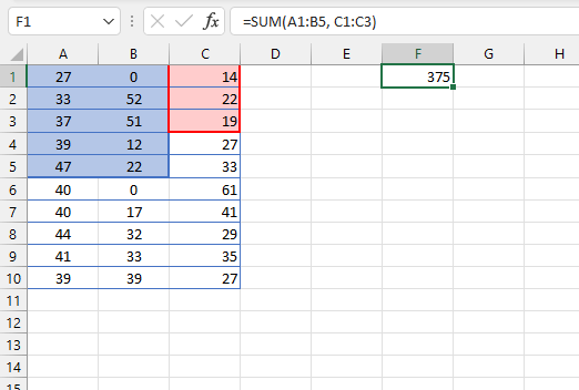
• If you entered the space character intentionally, the #NULL! response is an indication that the ranges you referred to do not overlap, and the result is therefore “null”. You can use IFERROR to hide this error message.

7. #NUM! error

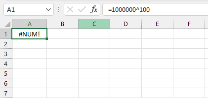
This response is not seen very often, but most people have encountered the #NUM! error in Excel at least once. The #NUM! error is usually displayed when the number is too large or too small, or when calculation is not possible.

The largest number that Excel can accommodate is 10³⁰⁸.

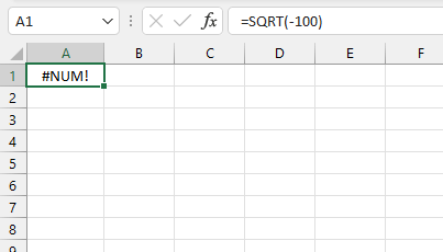
Another example: a negative number has no square root.

Possible solutions:

• Change the formula so that the value is within the range of valid Excel numbers.
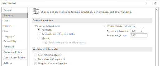
• Enable iteration calculation by going to File > Options > Formulas. This option will allow several attempts to find a solution when using formulas such as RATE, IRR, and XIRR.

8. #REF! error 

The #REF! error in Excel is displayed when the reference to a cell is invalid. This usually happens when a formula is built, and then a cell, row, or column which is referenced in that formula gets deleted.  

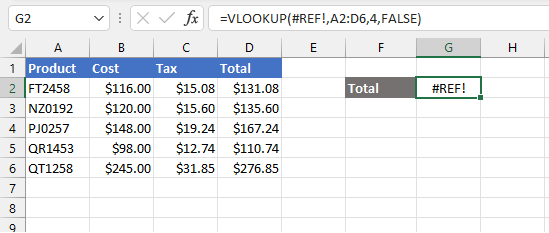
As you can see from the example above, not only is #REF! returned in the output cell, it also replaces the cell reference inside the formula itself, making it impossible to know exactly which cell was referenced.

A similar message will be returned if you copy and paste a formula to a location that makes the relative reference invalid.

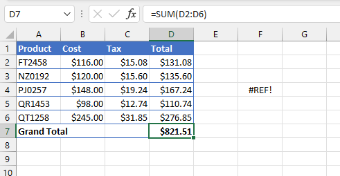
Since the formula in cell D7 refers to the five rows above, copying that formula to a cell that does not have at least five rows above will result in a #REF! error. 

Another reason for a #REF! error could be that the formula refers to another workbook that is closed.

Possible solutions:

• As a first resolution, try pressing Ctrl+Z on your keyboard (Command+Z on Mac keyboards) to undo the last action. This works fine if you just accidentally deleted a reference needed by the formula and want to restore your sheet to what it was before. By default, Excel allows you to undo up to 100 actions to an unsaved workbook.
• Using absolute cell references or named ranges will ensure that the original references are not shifted. Absolute references are made by placing dollar signs ($) before column names and row numbers.
• Check for, and open any other workbooks referenced in the formula.

9. #SPILL! error

#SPILL! errors in Excel are seen in the Dynamic Array Excel environment. This may refer to functions that are able to automatically return an output to multiple cells from a single input. A #SPILL! message is returned when one or more cells in the output area already contains a value, preventing an output.

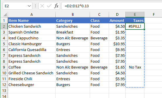
Possible solutions:

• Remove any obstructing values in the spill output range.
• Change the formula from a dynamic array formula to one that returns a single output and then copy the formula to the required cells.

10. #VALUE! error

What about when you see a #VALUE! error in Excel? 

• The most likely reason for this is that Excel found an unexpected character in a formula where it was expecting a number.

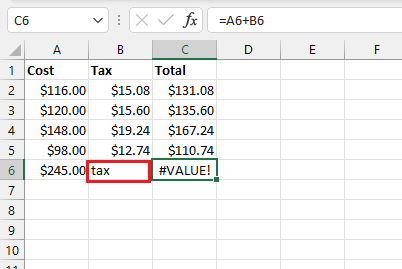
• Another possibility is that you are using an Excel function and an incorrect value type was submitted for one or more arguments. For example, if you are using VLOOKUP and enter a number less than 1 for the col_index_number argument, Excel will return a #VALUE! error. 

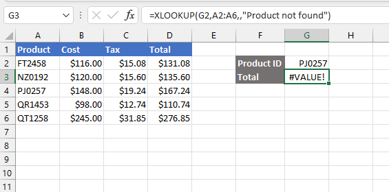
• For some formulas you will also get a #VALUE! error if you attempt to skip a required argument by entering a comma.

• #VALUE! errors also appear when you attempt to insert an array formula using the incorrect input method (i.e., you failed to use Ctrl+Shift+Enter). 

Possible solutions:

• Double-check the syntax rules for the function you are attempting to use. Check out our handy compendium of Excel function how-to’s here.
• Array formulas must be entered using the Ctrl+Shift+Enter method if using pre-Dynamic Excel.

How to hide errors in Excel

Sometimes it’s perfectly acceptable to get a non-mathematical response to your Excel formula. For example, #DIV/0!, #N/A, and #NUM! responses may be expected when certain types of data are being handled. If you prefer to return a friendlier response, or to perform an alternative calculation when Excel generates error messages, you may want to use the IFERROR or IFNA  functions.

=IFERROR(B3/C3,“”)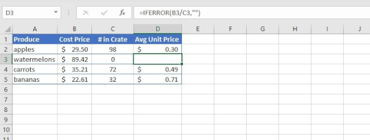

In the example above, the formula B3/C3 would have resulted in a #DIV/0! error. IFERROR was used to return a blank cell instead.

The IFERROR function applies to all the following errors: #CALC!, #DIV/0!, #N/A, #NUM!, #NAME?, #NULL!, #REF!, #VALUE! The danger, of course, is that you may end up hiding an error that you want to correct.

The IFNA function is similar to IFERROR, but it only catches #NA errors.

Key takeaways

1. Excel error messages provide clues to identify mistakes in a formula or value, which helps to debug and fix errors.
2. Common Excel errors include #DIV/0!, #N/A, #NAME?, #NULL!, #NUM!, #REF!, and #VALUE!
3. To fix these errors, we can adjust the column width, use IFERROR, check for formatting or syntax mistakes, or use formula auditing tools like Evaluate Formula and Error Checking.
4. It's essential to pay attention to error messages, which can help to improve your understanding of Excel functions.

If you want to improve your Excel skills in one hour and learn how to avoid common errors, check out GoSkills' resources, including expert-led courses on Microsoft Excel for you to learn at your own pace. GoSkills provides interactive and effective courses that cover a range of Excel topics, from basic formulas and functions to advanced data analysis and visualization.

Level up your Excel skills

Become a certified Excel ninja with GoSkills bite-sized courses

Start free trial