How to Create a Drop Down List in Excel

---

Excel drop down lists (or dropdown lists, if you prefer,) are an easy way to control the values which are entered in a cell. They are very user-friendly and are a great way to reduce input errors. 

You can make a drop down list in Excel in a variety of ways. We’ll explore how to create a drop down list in Excel using three methods.

Method 1 - Manually

If you want a simple option (for example, Black/White; Yes/No/Don’t Know, etc.), then the quickest method may be to do it manually.

1. Select a cell or range of cells where you want to create the drop down list.
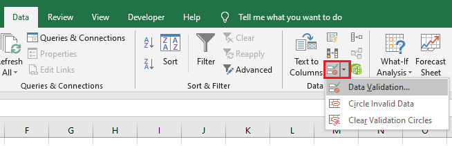
2. Go to the Data tab. Within the Data Tools command group, select the Data Validation icon.

3. In the Data Validation dialog box, within the Settings tab, select List as the Validation criteria.
4. In the Source field, enter the options, separated by commas. Make sure that the In-cell dropdown option is checked.

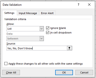
5. Click OK.

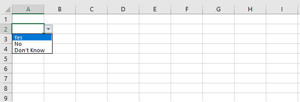
This will create a drop down list in the selected cells. All the items listed in the source field are listed in different lines in the drop down menu.

---

---

Method 2 - Referencing data from other cells

There is also the option to create a drop down in Excel using a range of cells as the source data for your validation list.

To do that:

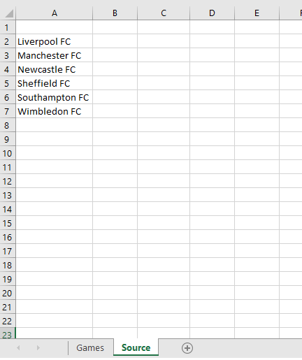
1. Of course, first, you'll need to set up a source, or list elsewhere. We’ve entered the source data in cells A2 to A7 on another worksheet named Source within this same workbook.
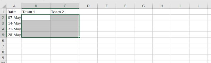
2. Next, select the cell or range of cells where you want to create the drop down list. In our example, we’ve selected B2:C5.

3. Go to the Data tab. Within the Data Tools command group, select the Data Validation icon.

4. Select ‘List’ as the Validation criteria.
5. In the ‘Source’ field, enter the range which contains the list of values to be used as your drop down list, or you can just click inside the ‘Source’ field and select the cells on the Source worksheet. 

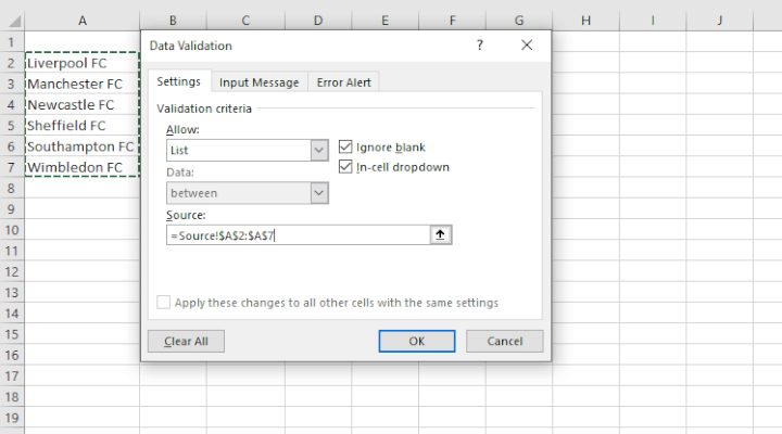
6. Click OK.

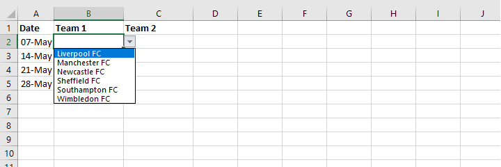
This will create a drop down list in the selected cell(s). Each item listed is shown in a different line in the drop down menu.

Method 3 - OFFSET formula (dynamic drop down lists)

You can also use the OFFSET formula to create dynamic drop down lists, which automatically update when items are added to the end of the list.

The syntax of the OFFSET function is:

=OFFSET(reference, rows, cols, [height], [width])

The first three arguments are required and the last two are optional.

• Reference - This is a cell or range of cells (adjacent) from which you can base the offset. Reference is the starting point. 
• Rows - This is the number of rows (down or up) to move from the starting point. If rows is a positive number, the formula moves downward from the starting reference. In the case of a negative number, it goes upward from the starting reference.
• Cols - The number of columns you want the formula to move from the starting point. As well as rows, cols can be positive (to the right of the starting reference) or negative (to the left of the starting reference).
• Height - The number of rows that the result should contain. If omitted, the height of reference is used.
• Width - The number of columns that the result should contain. If omitted, the width of reference is used.

To make this easier to follow, we’ll use the OFFSET function to create a dynamic drop down list in the following example.

We want columns B and C on the Games worksheet to display a drop down list of all the clubs within the league. The source data of club names will come from another sheet (Source) within this workbook. 

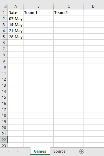
1. On the Games worksheet, select cells B2 to C5, since we want the drop down list to be created for all cells within that range.

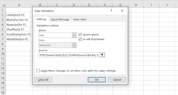
2. From the Data tab on the ribbon, in the Data Tools group, click Data Validation. The 'Data Validation' dialog box appears.
3. In the Allow box, click List.
4. Click in the Source box and enter the formula:

=OFFSET(Source!$A$2,0,0,COUNTA(Source!$A:$A),1)

The above formula tells Excel to use cell A2 in the Source worksheet as the starting point (note the absolute reference to cell A2). Since the result that we want should begin with the reference cell, the offset should remain at zero rows, and zero columns (away from the starting point).

The height of our result should be whatever the height of the list is, so we ask Excel to count the number of values within the list by using a COUNTA formula, making reference to the entire column A.

The result will be only one column wide, so 1 is the final argument in our formula. 

5. Click OK.

The drop down list works as seen in the two previous examples, but offers the added advantage of being updated whenever choices are added to the end of the list on the Source worksheet.

Simply add a new item to the end of the source list, and the drop down list choices will be updated immediately.

 

Allow other entries

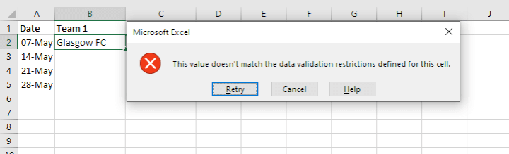
So far, we haven’t adjusted the Error Alert default for the drop down lists we’ve created. This means that once the list is set up, Excel will only accept the values which are a part of the list. If we try to type in a value that is not part of the Source list, we will get an error message. 

If desired, you can create a drop down list in Excel that allows other entries not included in the source list.

To do this: 

1. Select the cell or cells with drop down lists where you want to allow ‘on-the-fly’ entries.
2. Go to the Data tab, then from the Data Tools command group, click Data Validation.
3. The Data Validation dialog box will appear. Go to the Error Alert tab and uncheck the ‘Show error alert after invalid data is entered’ box. Click OK.

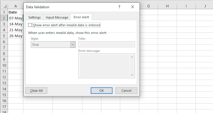You will now be able to enter a value that is not in the drop down list.

Copy data validation rule from another cell

If there’s a cell that carries a data validation rule that you’d like to copy to another cell: 

1. Go to the cell which contains the rule and copy.
2. Go to the target cell and from the Home tab, click the Paste drop down arrow.
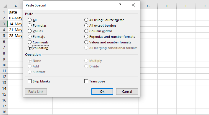
3. Choose Paste Special.
4. From the Paste Special dialog box, select the Validation radio button and click OK.

Add item to an Excel drop down list

Even if you’re not using a dynamic drop down list, here is a useful little trick to quickly add an item to a drop down list:

1. Go to the list and right-click one of the values.
2. From the context menu, click Insert.
3. Choose "Shift cells down" and click OK.
4. Type a new item.

The result is that Excel automatically expands the source range to include the first and last values in the list, and everything in-between.

Remove item from a drop down list

To quickly remove an item from a drop down list:

1. Go to the list and right-click the value to be deleted.
2. From the context menu, click Delete.
3. Choose "Shift cells up" and click OK.

The result is that Excel adjusts the source range so that the data validation source list starts with the reference to the first value and ends with the reference to the last value.

Remove a drop down list

If you want to remove all values from a cell, including drop down lists, formatting, etc., just go to the Home tab, click the Clear drop down, and choose Clear All.

However, if you only want to remove the drop down list but keep the values that were selected, do the following:

1. Select the cell(s) with the drop-down list.
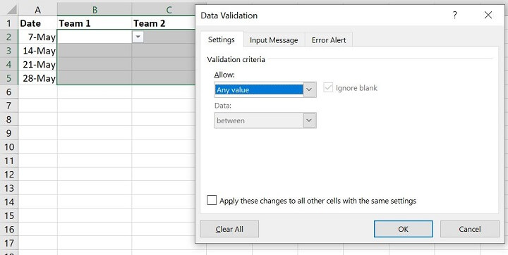
2. On the Data tab, in the Data Tools group, click Data Validation.
3. Under Allow, change List to Any value.

If you also want to remove all other drop down lists with the same settings, check "Apply these changes to all other cells with the same settings."

4. Click OK.

---

Create dependent dropdown lists

Here’s a twist. You may want to know how to make a dropdown list in Excel where the options change depending on what was selected in a previous dropdown list. 

For example, in column B we would select the name of the country whose league will be shown.

Then columns C and D would offer only those clubs which belong to the country selected in column B of that row.

Setting this up is as follows:

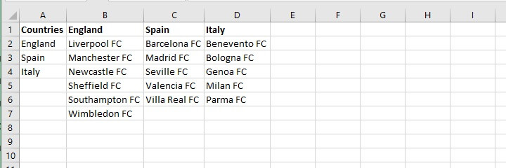
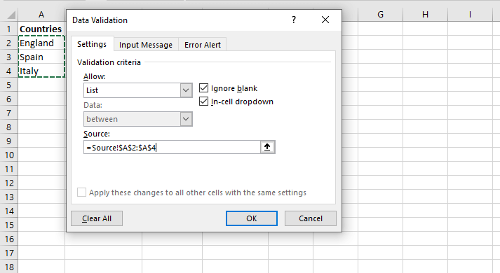
Step 1: Create a list of countries that will become your “parent” data validation list. We have listed England, Spain, and Italy as our parent list.

Step 2: List the club names by location in separate columns.  

Step 3: Create a named range for each country’s list, where the names are identical to your parent data validation list.

To display the parent list options in a drop down menu in Excel: 

1. Select the cell(s) where we want the parent list to appear as the drop down options. In our example, we have selected cells B2:B5. 

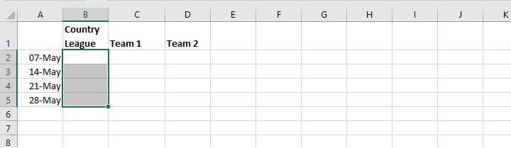
2. Go to the Data tab > click the Data Validation icon > click List from the Allow drop down > go to the Source field and select the $A$2:$A$4 range on the Source worksheet.

To display the dependent list options: 

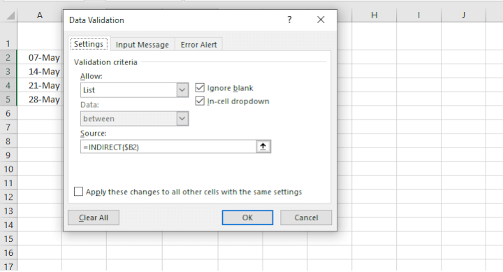
1. Select the cell(s) where we want the dependent values to appear as the drop down options. We’ve selected C2:D5.
2. Go to the Data tab > click the Data Validation icon > click List from the Allow drop down > go to the Source field and type =INDIRECT(B2).

In our case, we also want to use the same country league as the parent list for column D. Therefore, we should highlight the range C2 to D6 and use a mixed reference when entering the formula for the validation. 

Since we will always want to look in column B for the country name, the reference to column B is fixed but the row number will be relative to the row for which we are doing the selection.

We will therefore type =INDIRECT($B2)

Now our dependent lists in columns C and D work beautifully, with the options changing depending on what was selected in column B.

---

	Challenge me!
	Take this Excel super-challenge to test your skills in making dependent dropdown lists.

---

Learn more

Look at you, making drop down lists in Excel like a pro! Learn even more about Excel with GoSkills courses! You can try the Microsoft Excel - Basic and Advanced course. Or you can start with the free Excel in an Hour crash course today.

Learn Excel for free

Start learning formulas, functions, and time-saving hacks today with this free course!

Start free course