
The OFFSET function in Excel uses a specific reference point to return a reference to a cell or range of cells. It is often combined with other functions to build dynamic named ranges or dropdown lists relative to a specific cell or range of cells.
A dynamic range automatically expands and contracts to accommodate new or deleted data from the source. With dynamic arrays being built into the Excel 365 environment, OFFSET may be used a bit less frequently than before, but it is still important to understand how it works since some tasks are still best accomplished using this function.
Syntax
The syntax of the OFFSET function is:
=OFFSET(reference, rows, cols, [height], [width])
The first three arguments are required and the last two are optional.
- reference - a cell or a range of adjacent cells from which you base the offset. You can think of it as the starting point.
- rows - the number of rows to move from the starting point, up or down. If rows is a positive number, the formula moves downward from the starting reference. In the case of a negative number it goes upward from the starting reference.
- cols - the number of columns you want the formula to move from the starting point. Cols can be a positive number (to the right of the starting reference), or a negative number (to the left of the starting reference).
- height (optional) - the number of rows that the result should contain. If omitted, the height of reference is used.
- width (optional) - the number of columns that the result should contain. If omitted, the width of reference is used.
Get the free practice file!
Download the OFFSET practice file.
Basic usage
Here is a simple example of how OFFSET works.
=OFFSET(A1,0,1,4)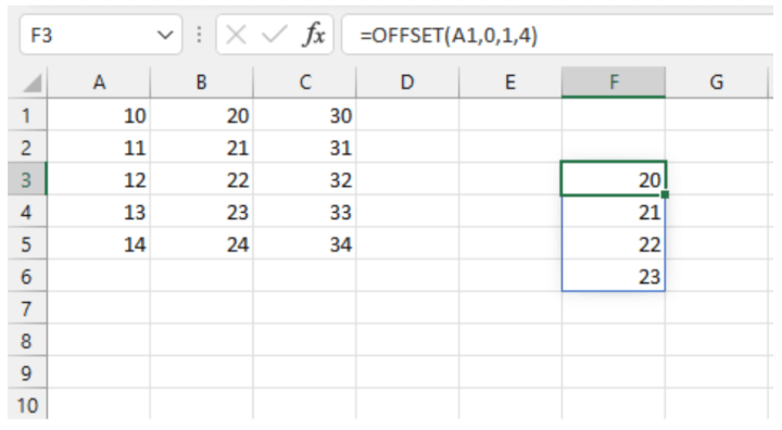
The formula in cell F3 uses cell A1 as our starting point, or reference. The second argument, 0, tells Excel to remain in the current row. A cols argument of 1 means to move one column to the right. These directions take us to cell B1.
The two optional arguments tell Excel what the dimensions of the array should be. The height should be 4 cells. So far, we realize that Excel will return the range B1:B4.
Since the final argument, width, is omitted, the width of the reference is used. In our example, A1 carries a width of one column, so there is no change to the B1:B4 range.
Using a range of cells for the OFFSET reference
As mentioned before, the reference argument may also be a range or array of cells. When this is the case, the position of the top left cell in the range is used to count the number of rows and columns in the row and cols arguments.
=OFFSET(A1:B1,1,0,3)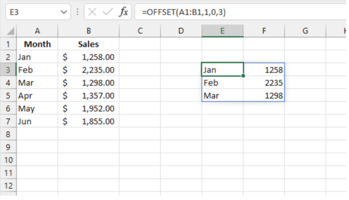
For the above formula, we move 1 row down from cell A1, remain in the current column, and copy three rows. The width of the output should be the same as the original reference (2 columns).
Using OFFSET optional arguments in Excel 2019 or earlier
If you are using a version of Excel before Microsoft 365, you may have noticed that your results look a bit different in some of these examples, specifically those where any of the optional arguments carry a value greater than 1. You will likely receive a #VALUE! error message, indicating that something is wrong with the way your formula was entered.
This is because prior to Excel 365, entering a formula in a cell meant that only a single output would be supported. If you wanted multiple values to be returned, you would either have to enter multiple formulas or enter an array formula. The steps are outlined below.
- Highlight the range of cells where the output should be displayed.
- Type the formula as usual, but importantly, do not press Enter.
- Press CTRL+SHIFT+ENTER (this is why array formulas are sometimes called CSE formulas) to let Excel know you are entering an array formula.
=OFFSET(A1,0,0,4,2)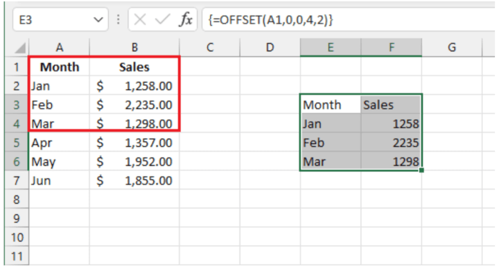
Excel automatically inserts curly brackets around the formula to remind you in future that this was entered as an array formula. (If you enter the curly brackets yourself, this will do nothing.)
Thankfully, the improved Excel engine eliminates the need to know the size of the output area since the environment is dynamic and will spill the results into as many cells as required.
OFFSET is a volatile function, so having several OFFSET functions within a workbook may cause your file to slow down noticeably.
OFFSET function example
OFFSET can be useful for calculating or returning a value that is relative to a certain location. For example, Excel does have an add-in to calculate the moving average of a list of values, but if we wanted to return a single value for the average of the last n values, OFFSET does the trick.
In the following Excel Table, Monthly_Sales, OFFSET can be used to calculate the average of the last three month’s sales.
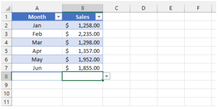
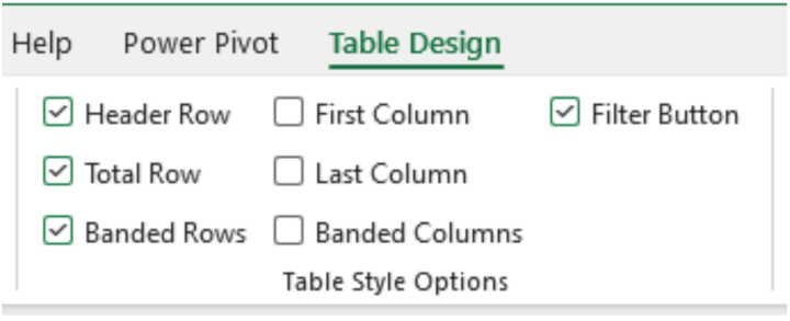
Note that the Total Row has been enabled.
Now we can use the structured reference of the total row to average the three cells immediately above.
=AVERAGE(OFFSET(Monthly_Sales[[#Totals],[Sales]],-3,0,3))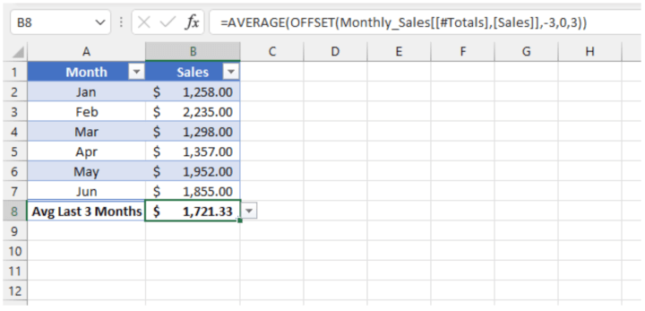
Whenever values are added for subsequent months, the formula in the Total Row will always use the values 3 rows above to calculate the average of the last three months.
Dynamic data validation (dropdown) lists
Data validation lists are often used as a way of reducing input errors by presenting a selection of values from a dropdown menu. If values are added to or removed from the source list, we naturally want the dropdown menu to be updated to reflect this change.
A combination of the OFFSET and COUNTA functions can be used to create dynamic dropdown lists so that the update is automatic, even if you are using pre-dynamic Excel. The formula looks like this:
=OFFSET(A1,0,0,COUNTA($A:$A),1)
An explanation of the formula is as follows:
- The second and third arguments being set to zero means that the dropdown list will begin with the value in cell A1 (the first argument).
- Using COUNTA($A:$A) counts the number of values in column A and fixes that as the height of the list.
- Using 1 as the final argument could have been omitted, since the formula will default to the width of the reference argument (in this case, it’s only 1 column wide).
Notes:
- Ensure that the values in that column are the only values you want reflected in your dropdown list. If there are any other values anywhere else in column A, they would also be returned, since the $A:$A portion of the formula refers to the entire column A.
- There are other options for creating dynamic dropdown lists in Excel, the most common being the use of the UNIQUE function, sometimes in combination with SORT and/or FILTER.
Ready to become a certified Excel ninja?
Start learning for free with GoSkills courses
Explore Excel coursesCreate a dynamic named range with OFFSET
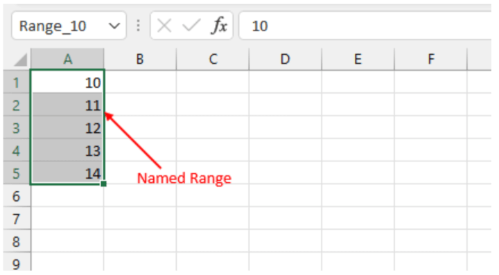
A named range is a range of cells with data that we want to use as a reference in formulas. Named ranges are often used as a simplified way of referring to a group of cells.
However, a problem arises when a formula refers to a group of cells by its named range, but values are later added to the source data. Unless the named range is redefined, any reference made to it will not be updated with the new information.
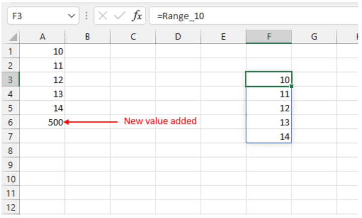
Obviously, it is not always practical to redefine the range whenever new information is added to the source. The answer to that is to make the range dynamic, in a way that is almost identical to the dynamic dropdown list solution above. To do this:
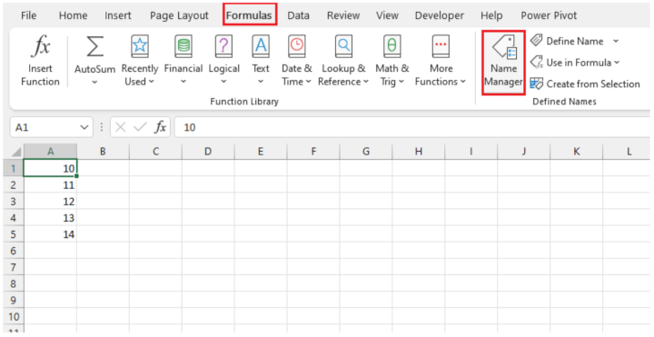
- Go to the Formulas tab.
- Click the Name Manager command.
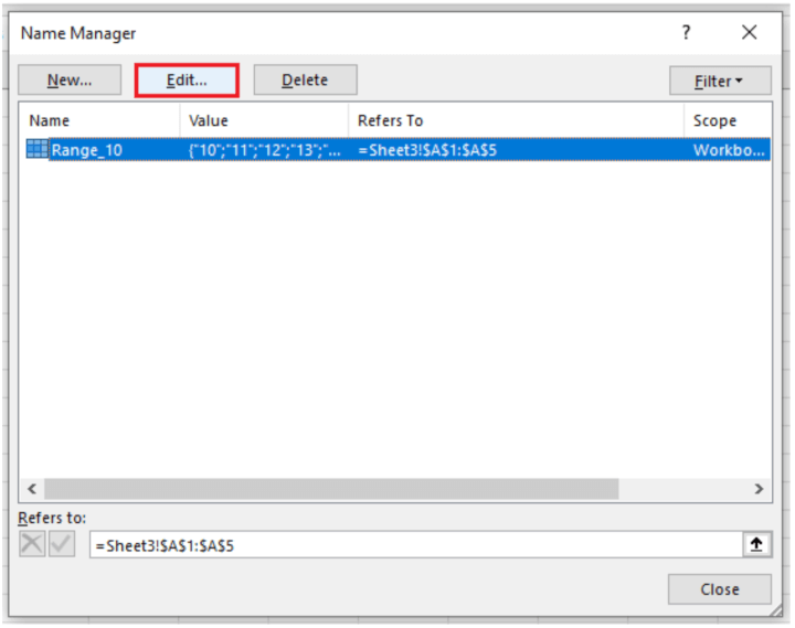
- In the Name Manager dialog box, select the Named Range you want to be dynamic and click Edit.
- In the Edit Name dialog box, note that Excel places the worksheet name in front of the cell reference in the Refers to: field. This is necessary, and ensures that the Named Range points to the correct group of cells, regardless of where in the workbook the Name is used.
- Update the Refers to: field to include the following OFFSET/COUNTA formula combination and click OK.
=OFFSET(Sheet3!$A$1,0,0,COUNTA(Sheet3!$A:$A),1)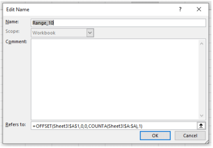
Get the free practice file!
Download the OFFSET practice file.
Troubleshooting the OFFSET function
Here are a few common errors when working with OFFSET:
- Slow worksheet. OFFSET is a volatile function, meaning that it recalculates each time the workbook opens or the worksheet changes. Having several OFFSET functions within a workbook may cause your file to slow down noticeably.
- REF error. If you get a #REF! error, this means you’ve made reference to an invalid range. For example, =OFFSET(A1,-1,1) will result in a #REF! error because the -1 argument references a row above Row 1, which does not exist.
- VALUE error. A #VALUE! error may result from entering the formula in an unrecognized format, such as failure to enter Ctrl+Shift+Enter in pre-dynamic Excel.
Verdict and final word
OFFSET might not be a function you use every day, especially since some of its features now come built-in with dynamic arrays, but it’s here for those times when you do need it. If you'd like to brush up your Excel basic and advanced skills, there are plenty of self-paced courses that make learning easy, engaging, and fun!
Ready to become a certified Excel ninja?
Start learning for free with GoSkills courses
Explore Excel courses