How to Use the Excel INDIRECT Function

---

Imagine an Excel function that, with a single argument, can add sophistication to your worksheet by allowing it to behave dynamically. 

It can take instructions from an input cell, incorporate them into formulas and display updated values or calculations as requested by the input cell. That’s what the Excel INDIRECT function does, and it’s a well-kept secret that you’re about to be let in on.

Syntax

Let’s start with the basics!

INDIRECT usually carries only one argument, and that’s a cell reference. There is an optional second argument in which you can type TRUE or FALSE. TRUE is the default. If you type FALSE it means you’re using the R1C1 cell reference style.

=INDIRECT(ref_text, [a1])

The vast majority of Excel users are familiar (and quite comfortable) with the A1 style of referring to cell locations. We won’t go too much into explaining R1C1 here, but it does deserve at least a brief explanation. 

---

---

R1C1 style

For example, in the A1 reference style, cell B5 refers to the second column/fifth row of an Excel spreadsheet. But the R1C1 cell naming convention refers to the row number first, followed by the column number. 

Cell B5 would be called R5C2 using the R1C1 style. In formulas, the R1C1 style uses relative references by telling Excel how far away the referenced cell is from the active cell. For example, R[-1]C means the cell value to be processed is one row above, in this same column.  

That’s R1C1 in a nutshell. We promised not to go into detail about how to use that now. That’s for another time and place. Right now, we’ll concentrate on the A1 style to keep it simple.

How INDIRECT works with cell references

To help you understand what INDIRECT does and how it works, take a look at the sheet below.

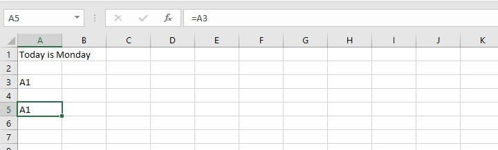Usually in Excel, we know that if you type EQUALS and a cell reference, Excel just copies and returns whatever is in that cell. In cell A5, we typed =A3, and as expected, Excel just copied the text that was in cell A3 and displayed A1. 

Let’s see how the INDIRECT function changes that.

=INDIRECT(A3)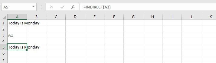

Now cell A5 says “Today is Monday.” 

The INDIRECT function used the cell reference within parentheses as instructions about what to do. In this case, the instructions said, “Display the value cell A3.” 

And since Excel knows that we are using the A1 reference style (optional argument is TRUE or omitted), the formula in cell A5 is indirectly saying =A1.

Now that we have gotten this far, I’ll bet you’re wondering, “That’s great, but how on earth is this useful?” 

We’re getting to that.

Using INDIRECT with named ranges

First, let’s use the INDIRECT function with named ranges. Here’s an example.

On this sheet, we have monthly sales figures of three items of produce. Just below, we want to be able to enter the name of a fruit in cell B7. And we want to have Excel perform the SUM, AVERAGE, MIN, and MAX functions by extracting the right values from the A1 to M4 dataset and return the results of the calculation in their respective locations.

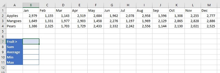Remember that we will want INDIRECT to find an input cell, in this case, cell B7. That input cell, in turn, gives instructions about a cell reference. But B7 won’t contain a cell reference. It will contain the name of a fruit, whether apples, mangoes, or pears.

By now you may have caught on. We can name cell range A2:M2 “Apples”, A3:M3 “Mangoes” and A4:M4 “Pears.” 

This is called creating a named range. To do this, simply select the range which your defined name will replace, and type the desired name in the Name Box at the upper left of the Excel worksheet (see below).

Once our named ranges have been defined, they will now act like cell references, so they’re ready to be used with INDIRECT. And that will be how we get our sheet to start behaving dynamically, depending on what’s typed in B7.

So if we wanted to find the sum of all mango sales, we would enter Mangoes in B7 and in B8, type:

=SUM(INDIRECT(B7))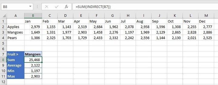

Another way to think about this would be to type:

=SUM(Mangoes)

in cell B8.

The result would be the same, but the problem with that approach is that we would also need to enter:

=AVERAGE(Mangoes)

=MIN(Mangoes)

=MAX(Mangoes)

We would need to type all four formulas each time we wanted to get the figures for each item of produce. When we use INDIRECT, we write the formula =SUM(INDIRECT(B7) once, telling Excel to look for the cell reference being queried in B7.

Using INDIRECT to return a text string

Here’s a fun fact. INDIRECT can also be used to copy exactly what’s inside a cell, instead of redirecting to another cell.

In cell A5 below, for instance, entering:

=INDIRECT("A3")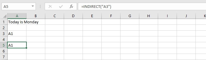

will return the text that is displayed in cell A3 instead of looking for more cell reference instructions in A3.

Now why would we want to do that, especially since we could have just typed =A3 without using INDIRECT at all?

Well, putting double quotes around an argument in the INDIRECT function says to Excel, “Treat this argument as a text string.” 

This now makes it a fixed value, so the formula will always point to A3 whether cells around it are moved, inserted, or deleted. Knowing this comes in handy in the following situations.

Use INDIRECT to refer to a different worksheet

We can use this principle to get INDIRECT to create dynamic worksheet references. 

For instance, if we have sales data for the last five years, with each year being on a separate sheet and carrying the same format, we can write a single formula on a query sheet to get information about any year we choose.

The idea is similar to the named ranges example we saw above. By entering a sheet name, Excel knows that we are not referring to the active worksheet. We need to specify which worksheet we’re looking to extract data from without hardcoding the worksheet name into the query sheet formula. To do this, we’ll use INDIRECT.

Cell B1 is going to be the variable input cell. The value in cell B1 will correspond to the sheet name. Excel’s format for referring to worksheet names is 'SheetName'!, so 

SUM('2016'!B2:M2)

will add values in the range B2 to M2 on sheet 2016. The trick will be finding a way to append the exclamation mark to the end of the year in the input cell so that Excel understands that a sheet name is being referenced. 

It helps to remember that the INDIRECT formula is looking for a cell reference to know what to do. If INDIRECT doesn’t recognize the argument as such, it will return an error.

That’s why we will insert the INDIRECT function into the SUM formula, and surround the non-cell references with double quotation marks. We also need the concatenation operator (&) to join the text elements to the cell references. Applying this, we get the following:

=SUM(INDIRECT("'"&$B$1&"'!B2:M2"))

As you can see above, the following elements have been enclosed by double quotation marks:

• Single quotes to denote a sheet name
• Exclamation mark and cell range

Additionally, these elements have been joined to the B1 reference with an ampersand on either side.

You may point out that the formula will also work without the single quotes around the sheet name, and it’s true. When a sheet name doesn't contain a space, Excel only needs the exclamation mark to identify it as a sheet name. 

But the above example was shown in case you run into this issue later. Plus, it doesn’t hurt to put the single quotes there every time. Instead of simply trying to memorize formats, it makes sense to understand why it’s done in a particular way so that you can continue to apply these principles as each situation arises.

Use INDIRECT to refer to a different workbook

We also use the above concept to refer to another workbook when using the INDIRECT function. The general format for referring to a range in another workbook is

=[WorkbookName.xlsx]SheetName!range

so

=SUM('[New Workbook.xlsx]Sheet1'!D39:D43)

will add values in the range D39 to D43 in New Workbook, Sheet1.

Since we’re now experts with the INDIRECT function, we can substitute whatever reference we like into the above formula by designating an input cell. In the example below, cell B1 is the input cell, and would contain the name of the sheet in the new workbook.

=SUM(INDIRECT(“'[New Workbook.xlsx]”&B1&“'!D39:D43”)

In all cases, the workbook being referenced must be open. Otherwise, INDIRECT will give a #REF error.

Use INDIRECT to create dependent dropdown lists

Another useful application of the INDIRECT function is to create dropdown lists where the options change depending on what is selected in a previous dropdown list. 

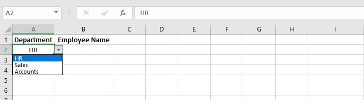
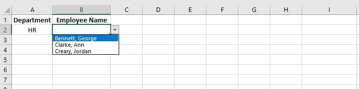
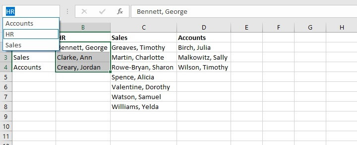
In the following example, cell A2 has a dropdown list containing three department names. Cell B2 contains another dropdown where employees’ names change, depending on which department was selected.

Setting this up is quite simple.

• Step 1: From the Data tab on the Excel ribbon, create a data validation list in a separate location using the department names. These will become the selection options for cell A2 (see below).

• Step 2: Create named ranges using these same list options, entering employee names for each department, as shown below.

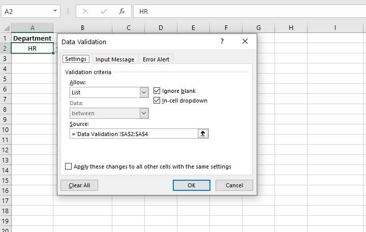
• Step 3: Create a data validation list for cell B2 with the formula =INDIRECT(A2).

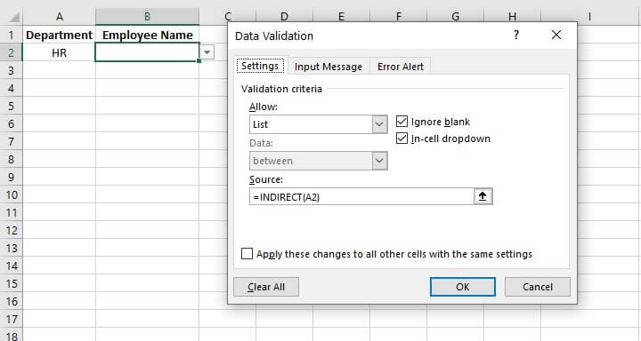The employee names will now change depending on the department selected in cell A2. 

Learn more

What do you think of the Excel INDIRECT function? What tasks will you use it to simplify? Sound off with a comment below!

And build up your Excel skills by trying our Excel - Basic and Advanced course. Try for free for seven days with our free trial and then upgrade to get access to a certificate for your resume.

Ready to become a certified Excel ninja?

Start learning for free with GoSkills courses

Start free trial