How to Use the FREQUENCY Excel Function

---

If you want to know how often the values within a certain range occur in a data set, you should consider using the FREQUENCY function in Excel. 

The FREQUENCY Excel function is an array formula, so its output spans multiple cells, and the method of input is slightly different from standard formulas.

Syntax 

The syntax of the FREQUENCY function is:

=FREQUENCY (data_array, bins_array)

• Data_array is the array (or list) of values for which you want to get the frequencies.
• Bins_array is the user-defined upper limits into which the values will be grouped.

FREQUENCY counts how often numeric values within certain groupings occur, so it isn’t useful for determining the number of text occurrences in a data set. To count how many times a certain text value occurs in a dataset, use the COUNTIF or COUNTIFS formula.

For instance, let’s look at how the FREQUENCY formula works using the example below.

---

---

How to use the FREQUENCY Excel function

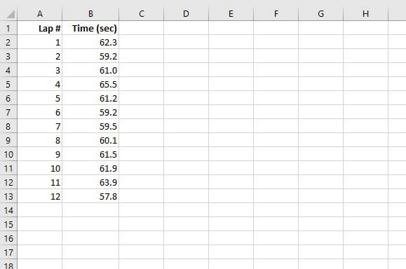
A racecar driver does time trials by doing twelve laps around the track. The time taken to complete each lap is recorded.

Step 1: Identify or create the data_array

The data array will be the area that contains the values that you will group and then count. In our example, this would be the number of seconds it takes to do each lap (cell range B2 to B13).

Now we can create a frequency distribution table based on the “bins” we create.

---

Step 2: Create the bins_array

Creating bins for the distribution table is all a matter of how you want your values to be grouped. In our case, we’ll create four bins or groups — 59, 60, 61, and 62 seconds.

These should be listed vertically somewhere on the worksheet.

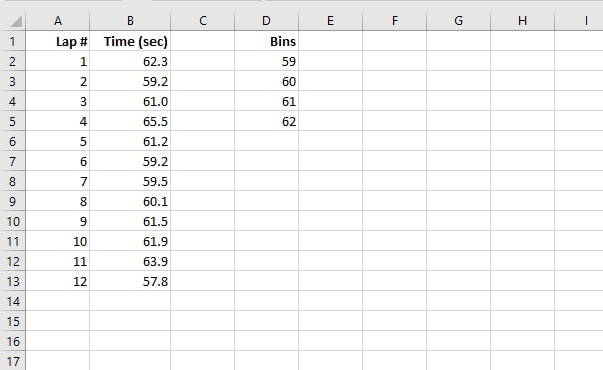We have entered our bins_array in cells D2 to D5.

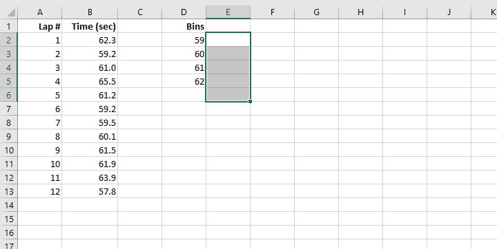
Step 3: Highlight the output area

Now we want to get Excel to count how many values fall within each group. As mentioned before, FREQUENCY is an array function, so we’ll need to select the number of cells that will be in the output area.

This means selecting one cell more than the number of bins. In the example above, the bins span four cells, so our output selection will be five cells. The output selection doesn’t have to be adjacent to the bins, nor even mapped directly across from it. But it usually makes sense to do that since this will make the table easier to read.

Exception: If you are using Excel 365 or Excel Online, Excel recognizes FREQUENCY as an array function. So there is no need to highlight all the cells in the output area. Simply go to the first cell of the output area and move on to Step 4.

Step 4: Enter the formula

While the cells are still highlighted, start entering the formula using the syntax outlined earlier.

=FREQUENCY(B2:B13, D2:D5)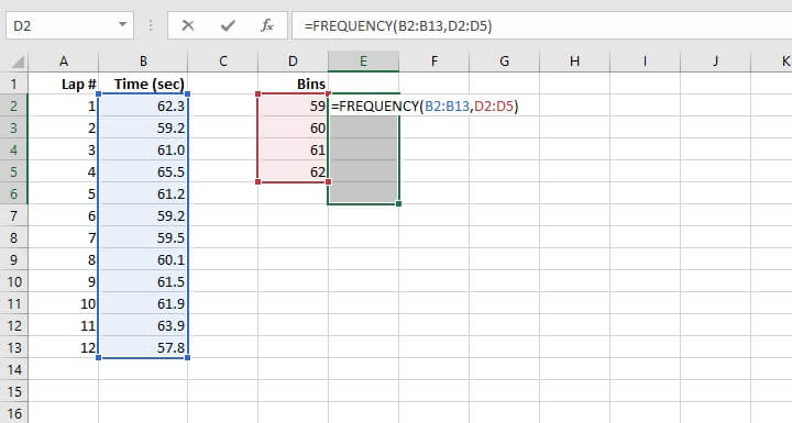 

Step 5: Submit the formula

This isn’t a standard formula, so it will not be submitted in the usual way. Array formulas are entered by pressing Ctrl+Shift+Enter simultaneously. On Mac devices, enter Control+Shift+Enter. For this reason, array formulas are sometimes also called CSE formulas.

Exception: If you are using Excel 365 or Excel Online, there is no need to enter Ctrl+Shift+Enter, because Excel recognizes FREQUENCY as an array function. Just press Enter as you would for any other function.

Step 6: Observe the output data

We can observe the following from the values returned in Column E:

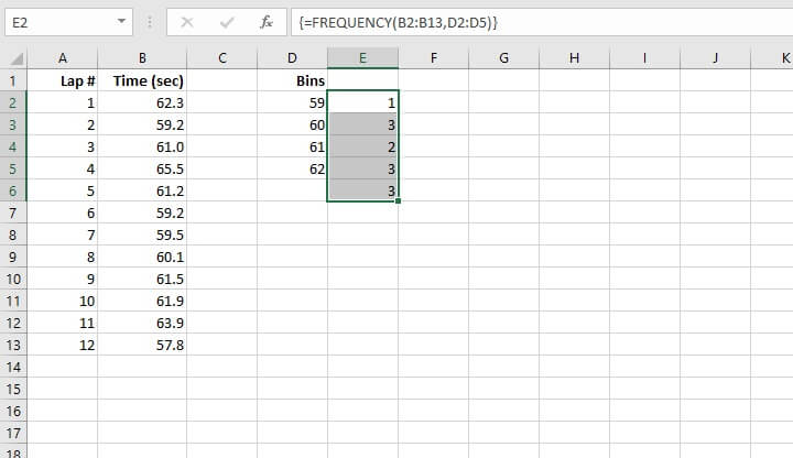
• Excel automatically inserts curly brackets { } around the formula to remind us in the future that this was entered as an array formula.
• There is one extra row of output data, that is cell E6. 
• Cells E3 to E6 have the same formula automatically displayed but are “grayed out” indicating that they were entered as an array formula and may only be edited from the first cell in the range (that is, cell E2).

Interpreting the output

It’s important to understand what our output is telling us, so let’s compare our results to the source data.

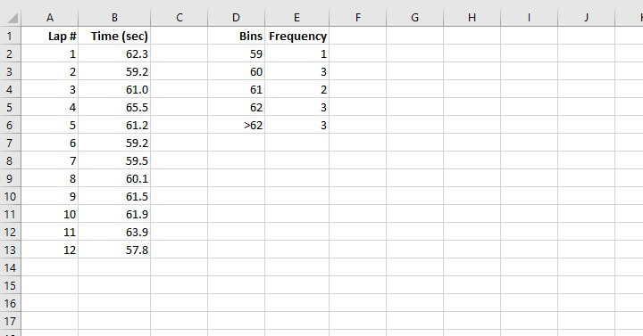
• We are told that bin “59” has a single occurrence. The first bin should be interpreted as occurrences up to and including this value. Our driver completed a lap in 59 seconds or less only once.
• Bin “60” has three occurrences. There were three laps completed in greater than 59 or equal to 60 seconds.
• Bin “61” has two occurrences. Two laps were completed in greater than 60 or equal to 61 seconds.
• Bin “62” has three occurrences. Three laps were completed in greater than 61 or equal to 62 seconds.
• The final output is considered an “Overflow” bin, where values greater than the last bin are collected. Three laps took longer than 62 seconds to complete.

Report frequency as a percentage

Reporting the relative frequency of each bin as a percentage is quite simple. We basically want to represent each value in Column E as a fraction of the total, or sum, of values. For this, we will use the following formula:

=E2/SUM(E$2:E$6)

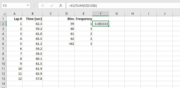We used a relative reference for the first reference to cell E2 because we want Excel to automatically change the reference for each respective row when we copy the formula to the cells below.

We used relative references for the range E2 to E6 since we want the reference to that range to remain in rows 2 to 6. In this case, an absolute reference ($E$2:$E$6) would have accomplished the same thing.

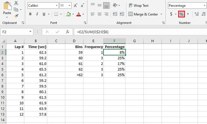
Once you’ve copied all the formulas down, select the F2 to F6 range and change the number format to Percentage.

Cumulative frequency percentage

You can report the cumulative percentage using the following formula:

=SUM(E$2:E2)/SUM(E$2:E$6)

When we lock the first reference to row 2, this is our way of anchoring the formula so that even when we copy to the cells below, Excel will always begin the SUM formula there.

Maintaining a relative reference to E2 is our way of creating an expanding range.

The reference to E2 to E6 is entered as a mixed reference because the denominator will always be the values in rows 2 to 6.

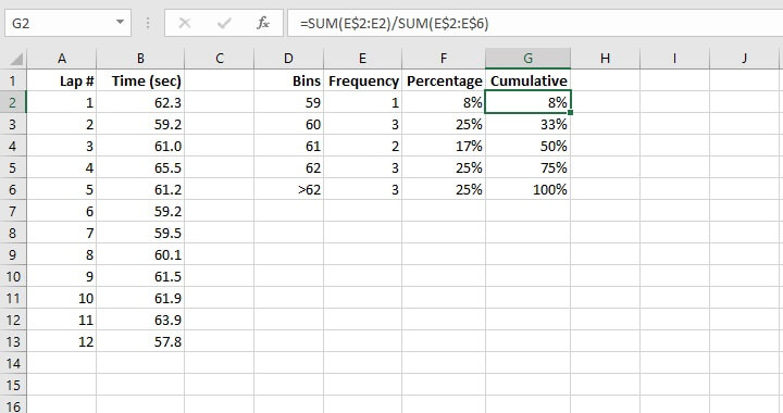When the formula is copied downward and the values are formatted as percentages, we get the output seen in the image above.

It can be seen from these results that the table created by the FREQUENCY Excel function can be (and in fact, often is) used in the creation of histograms and column charts.

Remarks

The frequency table created by this function is dynamic, so updates to the source data will result in an immediate update to the frequency table.

The “Overflow” bin can be labeled. In the example above, we might call it “>62”. However, changing the labels on the other bins will distort the results.

If you have blank cells or text in your source data, the FREQUENCY function will ignore that cell. That means it will not be treated as a zero or any other numeric value.

Learn more

The FREQUENCY function certainly simplifies the task of grouping values, especially in large datasets. 

Learn more about Excel functions with the GoSkills Basic and Advanced course!

Level up your Excel skills

Become a certified Excel ninja with GoSkills bite-sized courses

Start free trial