Sort Functions in Excel — How to Use SORT and SORTBY

Excel is a powerful tool designed to handle and organize data, allowing users to perform complex calculations, data analysis, and more. Working with data means you will want to place values in some kind of order – whether alphabetic, numeric, or some other custom order. The typical way of doing this is to use Excel's more traditional sort features. 

However, Excel sort functions are powerful tools for managing data dynamically. Once the formula has been applied to the dataset, no user intervention is needed when new elements are added—the data is automatically resorted, unlike the static "Sort" command in the Data menu. Used correctly, these functions can help you analyze and visualize your data more efficiently. 

What's the difference between SORT and SORTBY?

SORT		SORTBY
Only allows sorting by a single index (column or row) at a time.		Allows multiple layers of sorting.
The sort index is hardcoded as a column or row index number, which can lead to unexpected results if the dataset structure changes.		The sort index refers to a range, making column/row additions and deletions less problematic.
The data within the sorting index will be returned in the results.		Allows sorting based on a corresponding range, which may not be part of the results.

Based on the above comparison table, you might opt for SORTBY as it offers greater flexibility than SORT. However, if your dataset is relatively uncomplicated, SORT alone should adequately meet your requirements.

How to use the SORT function in Excel

The SORT function in Excel is a dynamic array formula that categorizes data in ascending or descending order. This function allows you to order a range of cells based on one or more columns and is very helpful when managing large datasets.

The syntax for the SORT function is:

=SORT(array, [sort_index], [sort_order], [by_col])

Arguments explained:

• array: The range of cells to sort.
• sort_index: The index of the column or row you want to sort by.
• sort_order (optional): 1 for ascending order (default),  -1 for descending order.
• by_col (optional): TRUE to sort columns, FALSE to sort rows (default).

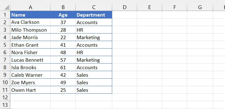
For example, let us imagine that you had the following list of employees, showing their names, ages, and departments.

You could sort the range A2:C11 by the second column (Age) in descending (largest to smallest) order with the following formula:

=SORT(A2:C11, 2, -1)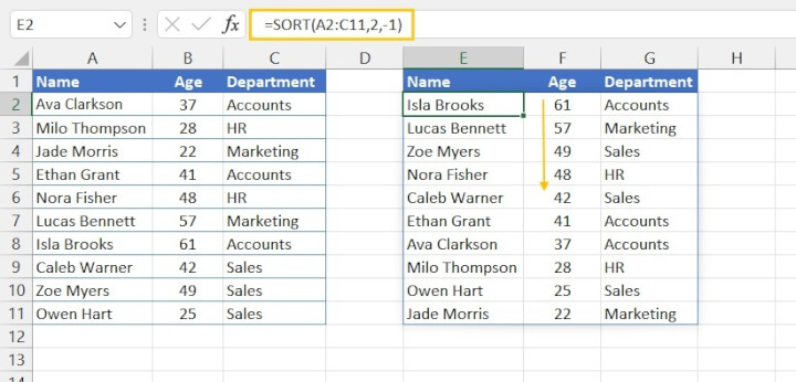

As with all dynamic array functions, there is no need to copy the formula to display all the results, as the SORT function in Excel automatically spills to the required number of cells.

In the above example, we omitted the final argument (by_col) because we wanted to sort the rows in our dataset, which is the default setting. Let's take a look at what would happen if we chose to activate the 'sort by column' setting instead by adding TRUE as the final argument.

=SORT(A2:C11,2,-1,TRUE)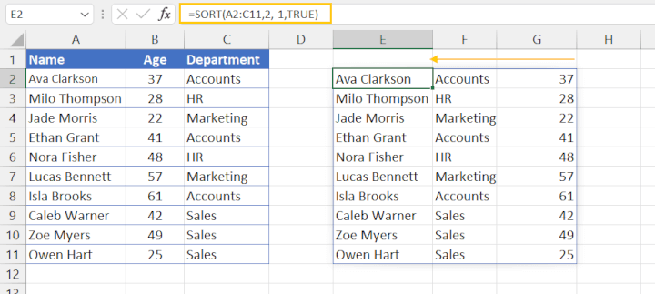

The result of this SORT formula is that the columns are now arranged in descending (right-to-left) order, with numbers ranked as smaller in value than letters.

How to use the SORTBY function in Excel

While SORT is a powerful tool, there are times when its sibling function, SORTBY, is needed. SORTBY is a function that dynamically accomplishes what the static multi-level sorting feature does in Excel.

The syntax for the SORTBY function is:

=SORTBY(array, by_array1, [sort_order1], [by_array2], [sort_order2],...)

Arguments explained:

• array: The range of cells to sort.
• by_array1, by_array2, ... (optional): The array(s) to sort based on.
• sort_order1, sort_order2, ... (optional): 1 for ascending order (default), and -1 for descending order.

For instance, given the same list of employees, we can sort using multiple columns, for example, using department as well as age. Here's how that can be done:

=SORTBY(A2:C11, C2:C11, 1, B2:B11, -1)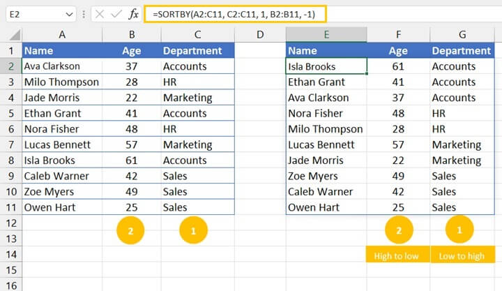

The above SORTBY formula first sorts the data by department in ascending order, then adds an additional layer of sorting by specifying that if there are multiple employees within each department, the names would appear in descending order of their ages.

The capabilities of SORTBY also mean that we can even sort by an array that will not be visible in the results. For example, what if we wanted to return the names of our employees in order of age without actually displaying their ages? Our formula would look like this:

=SORTBY(A2:A11,B2:B11,-1)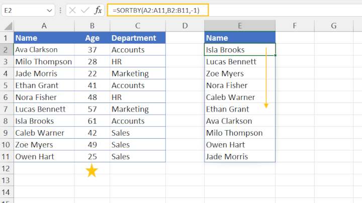

By establishing the array argument as A2:A11, only the names will be returned, even though we have used the range B2:B11 as the basis for sorting.

Advanced uses of SORT and SORTBY 

Knowing the basic usage of these functions isn't enough. Understanding how they interface with other features can make data analysis in Excel a breeze. Here are a few examples:

Dynamic data sorting

• The SORT and SORTBY functions are dynamic, meaning that if your dataset changes, your sort order will dynamically update. This is not the case with manual sorting, which has to be reapplied each time the dataset changes or new data is added. 
• Unlike manual sorting, the SORT and SORTBY functions leave the original dataset unaltered and return the result of the formula wherever it is entered.

Combining with other dynamic functions

• Combining the SORT and UNIQUE functions allows you to extract unique values from a dataset and sort the results, all in a single entry.

=SORT(UNIQUE(C2:C11))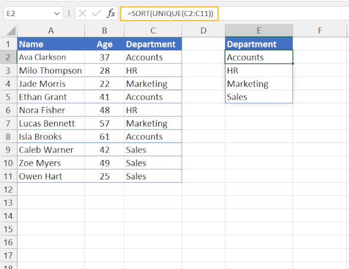

This simple formula extracts all the unique values in the C2:C11 range and sorts the results in alphabetic order.

• With a bit of imagination, we can use FILTER and SORTBY to effectively sort by a column we've chosen to hide from our display and return any columns of our choice.

=FILTER(SORTBY(A2:C11,B2:B11,-1),{1,0,1})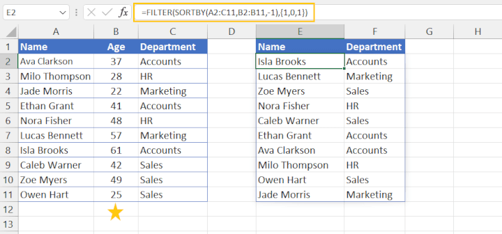

In the above example, the include argument of the FILTER function consists of 1,0,1 enclosed in curly brackets to denote "yes, no, yes" for whether each respective column should be returned. Consequently, the "Age" column is not shown, even though that column is used to sort the results.

Key points to remember

• These functions are only available in Excel for the web, Excel 365, or Excel 2021 and later.
• SORT only sorts arrays by the values in a single row or column, whereas SORTBY can sort arrays by multiple rows or columns.
• Since SORT and SORTBY are array functions, they return an array of results. Therefore, there must be a sufficient number of empty cells in the output area for the results to be returned. If one or more cells in the output area already contains a value, you will see a #SPILL error.

Conclusion

The SORT and SORTBY functions are incredibly powerful tools within Excel that can transform how you analyze and present large datasets. With this guide, you've gained an understanding of how they work, what parameters they require, and how best to apply them to your data. Remember, Excel is a diverse landscape, and the more you experiment and explore, the more proficient you'll become. A self-paced Excel course can help you improve your formula skills, critical thinking, and personal productivity. Happy sorting!

Ready to become a certified Excel ninja?

Start learning for free with GoSkills courses

Start free trial