PMT Function Excel

---

The Excel PMT function calculates payments for a loan based on constant payments and a constant interest rate. To calculate the payment amounts, the following variables must be known:

• The interest rate
• The total number of payment periods
• The value of all loan payments now (the loan principal).

 It is categorized with the financial functions within the Excel Function Library.

---

---

PMT function Excel 

Return value

The output from this function is the amount that the borrower can expect to pay at each interval (usually monthly), represented as a negative number (e.g., -$1,765.50). Of course, this does not account for taxes or fees which may be associated with your institution or locality.

Syntax

The syntax of the Excel PMT function is:

=PMT(rate, nper, pv, [fv], [type])

The first three arguments are required, while the two in square brackets are optional.

Arguments may be entered directly into the formula, or may be cell references containing the values.

Required arguments

The first example will look at how to use the PMT function with the three required arguments only.

To get a car loan of $12,000 at an annual interest rate of 6.49% over three years, the PMT function can be applied quite easily.

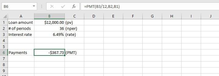The first thing to note in cell B2 is that the number of periods is entered as 36 (3 years x 12 months).

Secondly, the interest rate is entered in the PMT formula in cell B6 as the annual interest rate divided by 12. This is because since the loan period has been broken down into monthly payments, the interest rate must also be entered as a monthly rate in the loan calculator. Otherwise, it would seem that the interest of 6.49% is being applied to the loan every month.

Since no optional arguments were entered, the assumption is that at the end of 36 months, if all payments are made as agreed, then the loan is considered paid off and has no further cash value. It is also assumed that payments are due at the end of each one-month period.

Finally, as mentioned before, the return value is shown as a negative value since it is money being paid by the borrower.

In cases where a deposit is required, the present value is calculated as the loan amount less the deposit. Therefore, only the amount that is actually disbursed is used in the PMT calculator.

Let’s now learn how to apply the two optional arguments in the Excel PMT function.

Future value

The future value (fv) argument is typically used to calculate the amount of money to be deposited at each interval to achieve a certain return at the end of an investment period. The interest rate must be known.

For instance, if an interest rate of 7.5% is offered on 5-year investments, and we would like to have $2,000 at the end of five years, how much would we need to invest each year?

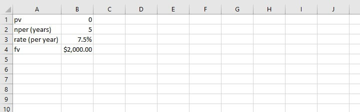In this case, the number of periods (nper) and the interest rate (rate) are both in the same units (years), so there will be no conversion to months. The present value (pv) is zero, since we are starting out with no money in the investment account.

=PMT(B3,B2,B1,B4)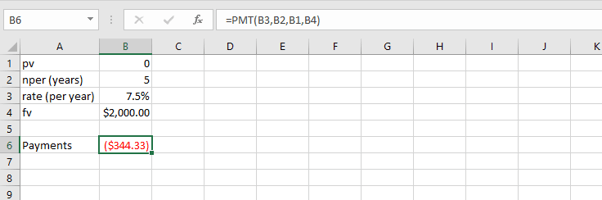

The “type” argument is omitted, so the expectation is that payments are due at the end of each period. The PMT calculator has determined that annual payments of $344.33 for five years at an interest rate of 7.5% will yield a return of $2,000.

Payment type

What if payments are expected at the beginning of each year rather than at the end? Then we would type 1 as the last argument of the formula. When payments are made at the end of a period, we can either type 0, or omit that argument.

=PMT(B3,B2,B1,B4,1)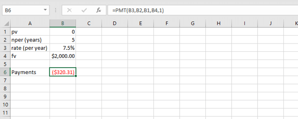

The annual payments to get a $2,000 return are now less because interest is being applied from the beginning of each period.

IPMT, PPMT, and PV functions

Closely related to PMT are IPMT, PPMT, and PV functions. The IPMT and PMT functions are used to calculate interest and capital repayments for each repayment period. They help us understand how the proportions of interest and capital repayments change over the life of the loan.

The PV function is used as a reverse calculator for calculating present value. 

IPMT function

The syntax of the IPMT function is:

=IPMT(rate, per, nper, pv, [fv], [type])

Let’s return to our car loan scenario.

Assuming that we have been making repayments on time, how much of the $367.73 payment is going toward interest in the first month?

=IPMT(B3/12,1,B2,B1)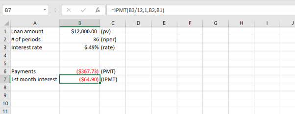

The figure in cell B7 shows the portion of the loan payment which will go toward interest. The difference will be applied to the principal.

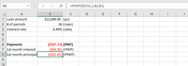
PPMT function

The PPMT function can be considered the opposite of the IPMT. It is used to calculate the principal portion of a loan payment. The syntax of the PPMT function is:

=PPMT(rate, per, nper, pv, [fv], [type])

In our previous example, we could have subtracted the interest amount from the loan payment amount, or we can use the PPMT function.

=PPMT(B3/12,1,B2,B1)

The IPMT and PPMT functions are useful for charting and observing how the proportion of interest changes over the lifetime of a loan. An example is illustrated below.

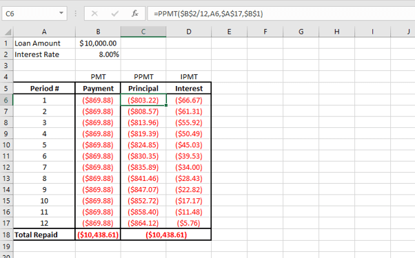Note that relative and absolute references have been applied where appropriate to make the copying of formulas easier in the creation of the chart.

The chart visually illustrates the increasing proportion of the repayments being applied toward the principal amount, and the related decrease applied to interest.

PV function

Conversely, if the borrower knows how much they can afford to pay per period, then the PV function can be used to calculate the present value of their payments as a lump sum. In other words, the value of the loan they can get now.

The syntax is:

=PV(rate, nper, pmt, [fv], [type])

If the bank’s interest rate is 12% for a 3-year loan and the borrower is willing to pay $1,000 per month, the PV can be calculated. Let’s enter the values directly into the formula.

=PV(12%/12,36,-1000)

Note that the pmt argument is entered as a negative number (-1000).

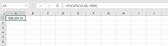With the information provided, the present value of this loan would be $30,107.51.

Learn more

Now that you’ve seen how Excel can demystify this seemingly complex topic, why not download our practice exercise and experiment with some scenarios of your own? 

Then, you can really roll your sleeves up by checking out our course library for even more Excel tools to enhance your workflow. You can start with the Microsoft Excel - Basic and Advanced course today!

Level up your Excel skills

Become a certified Excel ninja with GoSkills bite-sized courses

Start free trial