How to Make a Table in Excel

In everyday speech, a data table is simply an arrangement of rows and columns. In Excel, however, a table is something very specific. Excel tables are special data sets that work dynamically as a single unit, and have special commands and features to manage their contents.

What is an Excel table?

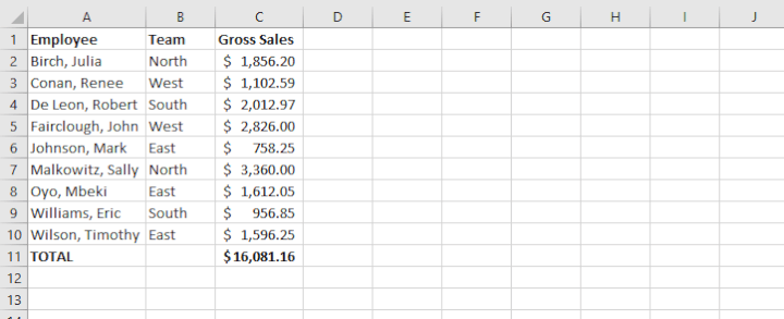
Below is a normal cell range in Excel.

Below is the same data, in an actual Excel table.

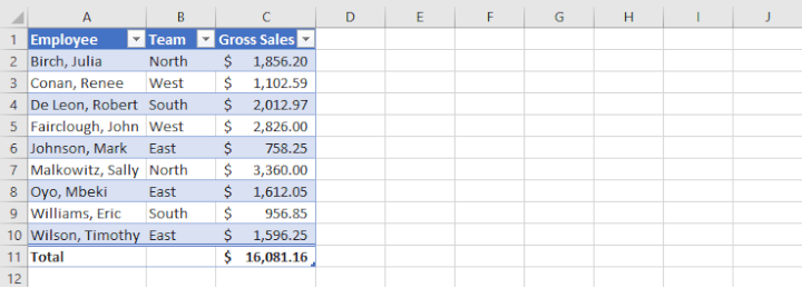
The real differences are explored below.

Features and benefits of Excel tables

So why choose tables over plain ranges? Excel tables aren’t just about looking pretty. They behave differently from basic ranges and have unique features and functionalities. Some of the benefits of Excel tables are:

• They expand and contract automatically as you add or remove rows and columns. This is called ‘dynamic’ behavior.
• The column headings in Excel tables remain visible while scrolling.
• Their drop-down lists and interactive slicers make it easy to sort and filter data.
• They have specially-formatted formulas that automatically include the table name and other elements instead of cell references.
• Excel comes with pre-designed table styles.
• You have the ability to sum, count, average, or find the minimum and maximum values in a data set with a simple click of the mouse.

How to create a table in Excel

With all of their features, you’d think that making a table would be complicated. It’s not. In fact, it’s surprisingly easy. To convert a plain range of cells into an Excel-formatted table, just follow the steps below:

1. Select any cell within your data set.
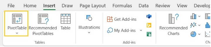
2. From the Insert tab, go to the Tables group and click the Table button.
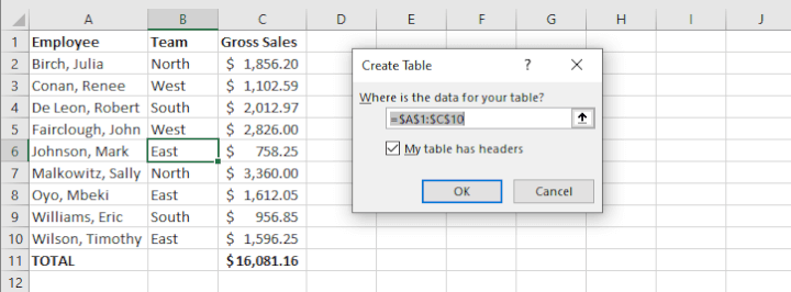
3. The Create Table dialog box appears with all the data selected for you automatically. Excel is usually able to identify where your data starts and ends. Otherwise, you can adjust the range as needed. If your first row contains headers for your data set, make sure the ‘My table has headers’ box is selected.
4. Click OK.

Excel will change the range to a table using a default style, which you can change at any time.

Shortcut alert: You can format as a table even more quickly by using the Ctrl+T shortcut on both Windows and Mac keyboards.

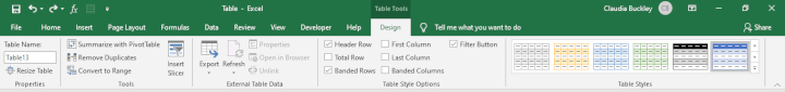
A new tab, the Design tab, also becomes available on the Ribbon. This Table Tool is called a contextual tab because it is activated only when a table is selected and carries commands specific to tables. If you click outside of the table area, the Design tab goes away.

Create a pivot table

Pivot tables are special types of tables, fantastic tools for condensing and summarizing massive amounts of data into manageable amounts. Commands for working with pivot tables are found on the Insert tab of the Excel ribbon. 

Steps for working with pivot tables are explained in more detail here.

Rename an Excel Table

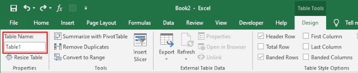
Each Excel-created table is given a default name, which can be viewed in the left corner of the Design tab when the table is selected. The first table in a worksheet is named Table 1. 

It’s a good idea to change the name to something meaningful so that it will be easier to identify and work with the table later. To change a table name:

1. Select any cell in the table.
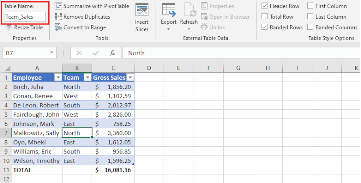
2. Go to the Table Name field on the Design tab.
3. At the far left of the Ribbon, click in the Table Name field.
4. Type in a new name, and press the Enter key.

Note the following rules when naming Excel tables:

• The table name can be up to 255 characters long.
• The first character of a name must be a letter, underscore ( _ ), or backslash ( / ).
• The other characters in the table name can be letters, numbers, underscores, or periods.
• Space characters are not allowed as part of a name.
• Names can't look like cell addresses, such as A1 or R1C1.
• A table can have a single character as its name - except for the letters C, c, R, r .
• Names are not case-sensitive. For example, Sales and SALES are treated as the same name.

We’ve named our table Team_Sales.

Change a user-defined table name

If you want to change the name you’ve given to a table, just return to the Design tab and overwrite the old table name with the new name. Hit Enter, and you’re done.

Delete a table name

All Excel tables must have a defined name. So you can’t actually delete a table name, but you can rename it, as we saw above. The only way to truly delete a table name is to convert the table to a cell range.

Convert a table to a range

To convert an Excel Table to an ordinary range:

1. Select any cell within the table
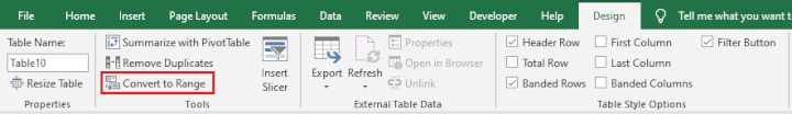
2. Go to the Design tab
3. From the Tools command group, choose the Convert to Range command.

4. A pop-up will ask, “Do you want to convert the table to a normal range?” Click OK to confirm.

This will remove the special table tools and behavior, and any cells which previously contained structured formulas will be converted to absolute cell references.

Show totals in a table

To summarize the data within a column, Excel has a built-in command to display the total at the end of a table.

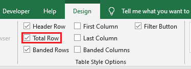
Just click any cell within the table, go to the Design tab and check the Total Row checkbox within the Table Style Options command group.

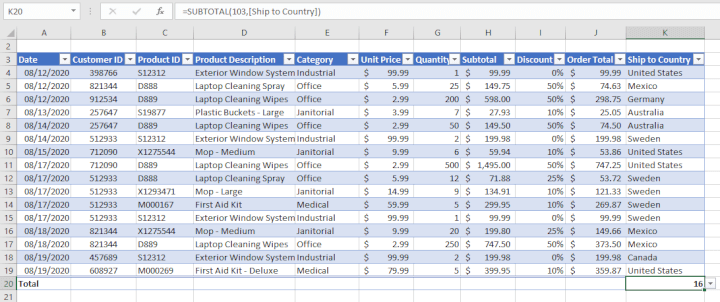
A Total Row will be added at the bottom of the table, and Excel will choose one or more columns and display their sum, count or some other type of numeric summary. Excel chooses the summary formula depending on how it assesses the data type.

In the following example, the Total Row option was checked, and Excel counted the number of orders by using SUBTOTAL function 103, which maps to the COUNTA function.

In the above example, Excel counted the number of orders by using SUBTOTAL function 103, which maps to the COUNTA function.

Change and add totals

You can add totals to columns, or change the formula Excel has chosen for a column quite easily, by doing the following.

For example, to display the total to be collected from all the orders, go to cell J20 and click the dropdown arrow.

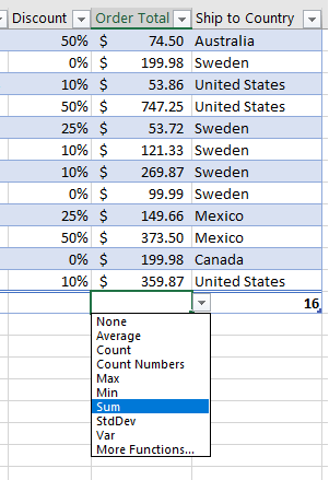
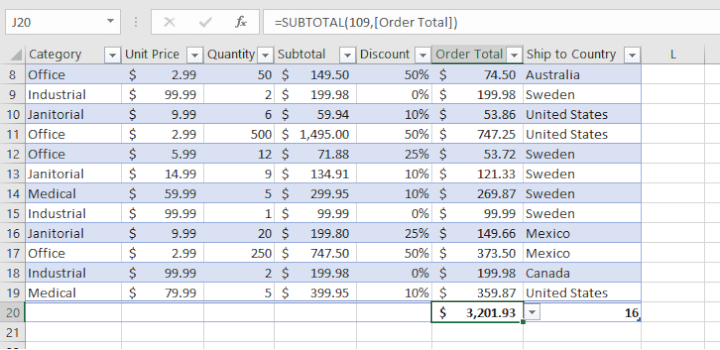
Select the function you want to be used (in this case, we’ve chosen the Sum function). The appropriate SUBTOTAL function will be inserted and the relevant value will be calculated based on the visible cells in the table. 

If none of the SUBTOTAL functions summarizes the column the way you want, any valid Excel function may be inserted. For example, to determine the number of different (unique) countries to which orders will be shipped, we can use the 

=SUMPRODUCT(1/COUNTIF([Ship to Country],[Ship to Country])) formula.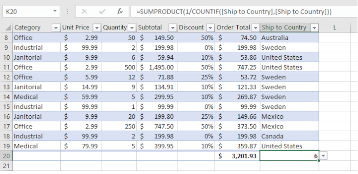

Of course, if you have Excel 365, the UNIQUE function is available to take care of this even more easily

Notice that the structured format of formulas in Excel tables may take a bit of getting used to at first. However, this is what allows the table to behave dynamically without being restricted to absolute cell references. 

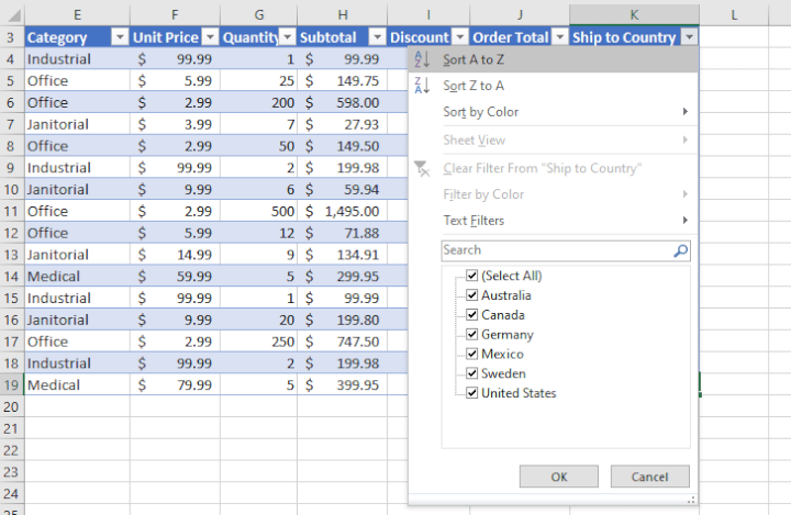
Sort and Filter Data

The dropdown arrows on the table header names can be used to sort or filter data. These work the same way as the Sort or Filter commands from the Data tab would work on a plain range, the main difference being that they are available right there in the data table, without having to navigate back and forth between Ribbon commands.

Slicer

Another feature available with data tables in Excel (starting with Excel 2010) is the interactive Slicer, which allows you to filter data visually. Follow these steps to access the Slicer:

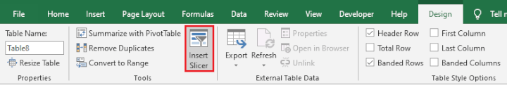
1. Click the table.
2. Go to the Design tab .
3. Select Insert Slicer from the Tools command group.

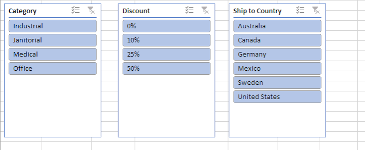
A dialog box with all the heading names will appear. From here you can check the boxes which allow grouping of values in the data table.

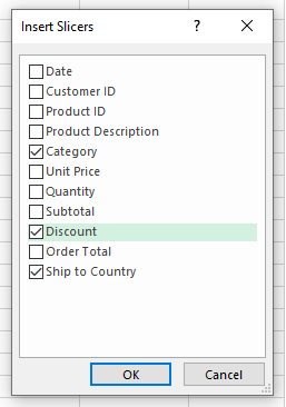
The slicers will then appear as objects within the worksheet, which may be arranged to your convenience by dragging them to a location which makes them easy to work with.

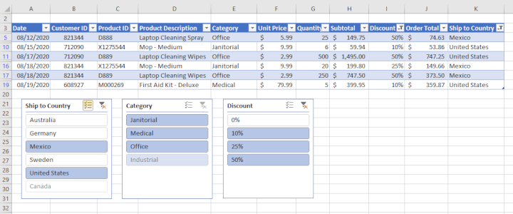
The slicer labels act as filter options for the data set. For example, to view orders being shipped to Mexico to which any discount was applied, click Mexico on the Ship to Country slicer, and on the Discount slicer, either click the Multi-Select command, then select the 10%, 25%, and 50% labels; or select those same labels while holding down the Ctrl key.

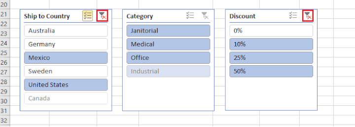
Click United States, and both the Mexico and US shipments with discounts applied will be shown. Any label which isn’t applicable will be grayed out and not available for selection.

To clear filters and redisplay all values in a category, select the Clear Filter icon at the top right of each slicer.

To remove the slicer objects from your worksheet, click on each slicer, and with the handlebars displayed, press the Delete key.

Change table style

To change your table from the default style, select any cell within the table then go to the Design tab. 

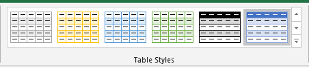
Choose a desired style from the Table Styles command group, using the scrollbar to see all the available options.

Help! My Excel data table isn't working.

When you’re using Excel tables, here are two lesser-known tips that might help ease your frustration:

• If you notice that your table isn’t expanding automatically when you add a row or column, you may need to unprotect your worksheet.
• You can't copy or move multiple worksheets if any of the sheets contains an Excel table.

Final notes

Excel tables aren’t as intimidating as they may have seemed at first, right? In fact, they’re actually designed to simplify your Excel workflow. Why not take our free Excel in an Hour course to get up to speed on our recommended Excel basics?

Learn Excel for free

Start learning formulas, functions, and time-saving hacks today with this free course!

Start free course