Using AutoFill in Excel

Entering predictable or repetitive data in Excel is zero fun, and may leave you wondering if there's a way to speed up the process.

Great news: there is! Excel's AutoFill feature suggests that you can set up your document to predict data patterns, allowing the cells to fill themselves in along the way.

And hey, any work that completes itself gets my vote.

 

 

What is AutoFill?

AutoFill is Excel’s way of being your smart little assistant who knows exactly what you want to be done next, and does the legwork for you. It’s a catch-all way of describing various built-in features which save keystrokes and time by picking up on patterns and filling in values to reduce manual entry. 

Ways to autofill in Excel

AutoFill shows up in different ways - sometimes by copying a formula to adjacent cells, at other times completing a list of days or months, or even by observing a formatting pattern and applying it to empty cells. Ready to learn how to recognize when Excel is giving you a helping hand?

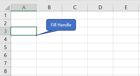
The Fill Handle

Every active cell (that’s the one that your cursor is currently sitting in) has a Fill Handle. This is a small green square at the bottom right corner of the active cell.

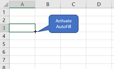
When you hover over the Fill Handle, the pointer changes to a small black plus sign.

Dragging or double-clicking on the Fill Handle will activate AutoFill

This feature is useful for copying values or formulas to adjacent cells.

Use the Fill Handle to copy the same value

The Fill Handle can be used to replicate a value simply by going to the cell which has the desired value and dragging the Fill Handle to the cells where you want that same value to appear. This works whether the cells within the range to be filled were empty or they contained values. If they have values, those values will be overwritten.

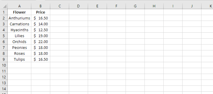
To illustrate how this works, take a look at this list of flowers and their prices.

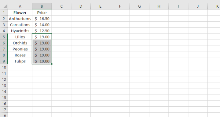
If we go to cell B5 and drag the Fill Handle all the way to cell B9, the prices of orchids, peonies, roses, and tulips will now be changed to $19.

Use the Fill Handle to auto-populate values in a series

At other times there's an obvious pattern that needs to be completed. The pattern may be a trend in numbers, days, or months that increase or decrease by a certain value. In this case, you'd probably rather have it auto-populate than subject yourself to the tedium of manual entry.

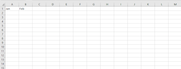
On the worksheet below, we’ve entered “Jan” in cell A1 and “Feb” in cell B1. 

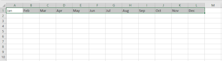
We’d like to enter the remaining months of the year in the columns to the right. All we need to do is highlight both cells A1 and B1, then drag the B1 Fill Handle until we get to "Dec."

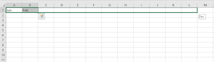Because we made cell A1 our active cell, Excel recognizes that “Jan” followed by “Feb” most likely refers to the “January, February…” series. This establishes the beginning of a pattern which our assistant uses to finish up the task.

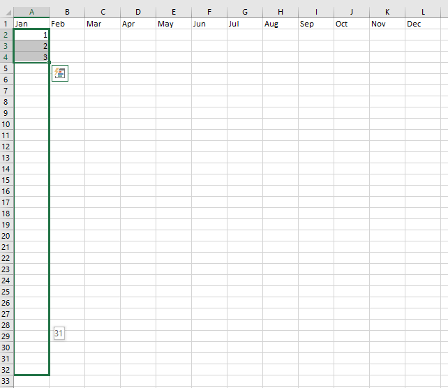
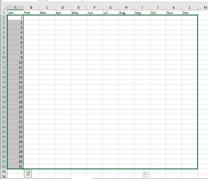
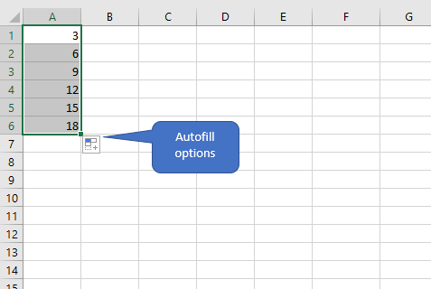
Now we’re on a roll. Let’s enter the first few numbers in a series and use AutoFill to copy them to the empty cells.

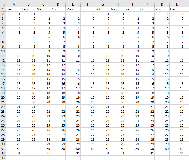
And we can duplicate these values by using AutoFill to copy across to Column L. 

Of course, we’d need to delete a few extra days from some months, but you get the idea. Not having to type those numbers in one-by-one saves you serious time (and possibly, your sanity).

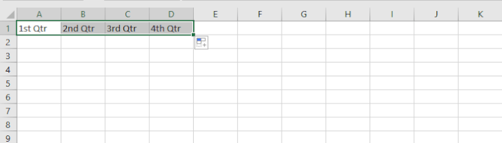
Excel can pick up on other kinds of patterns too, like this one:

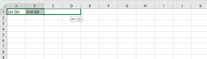Just highlight, drag, and release. AutoFill completes the series by filling in the third and fourth Quarters.

Use the Fill Handle to copy formulas

Instead of pressing Copy and Paste when you want to copy a formula to adjacent cells, AutoFill again comes to the rescue. The Fill Handle teams up with the principle of relative, absolute, and mixed cell references to figure out what portion(s) of a copied formula should be identical to the original, and what portion(s) should be relative to the row and column in which it is located.

Notice that in the case above, Excel is also smart enough to detect where your data ends, so the double-clicking method worked. If there are gaps in your data that make it difficult for Excel to recognize where the data ends, you may have to drag to the end of the dataset.

Autofill when entering formulas

Speaking of formulas, have you ever noticed that when you start typing in the first few letters of an Excel function, Excel suggests a list of functions that start with the letters you’ve typed in? If you press the Tab key, Excel will complete the name of the first function on the list, and the open parenthesis. Alternaively, you can arrow down to the one you want, press the Tab key, and finish up by entering the arguments and closed parenthesis.

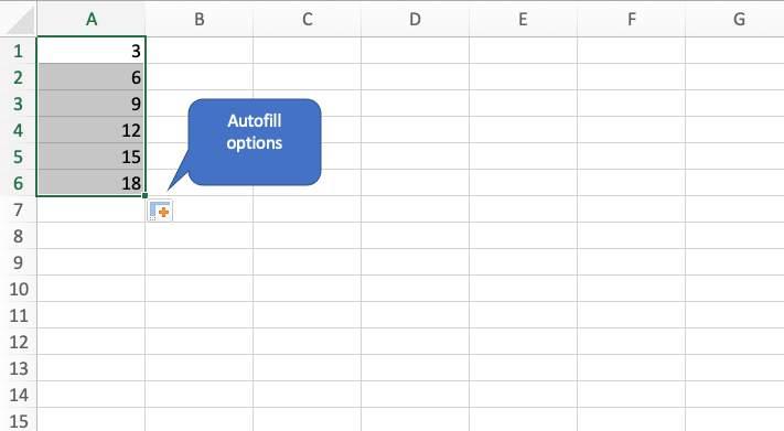
AutoFill options

You might have noticed the little icon to the lower right of the Fill Handle after you’ve executed an AutoFill command. 

 

If you’re using a Mac, it may look like this:

What does it do?

When you click on that icon, you’ll see some options which allow you to override the action taken by the AutoFill feature, including:

• Copy Cells (for when you just want to duplicate what’s already there)
• Fill Series (for continuing a trend)
• Fill Formatting Only (only copy the format)
• Fill Without Formatting (copy the value or trend but not the format)
• Flash Fill (Wizardry! More on that later!)

 

 

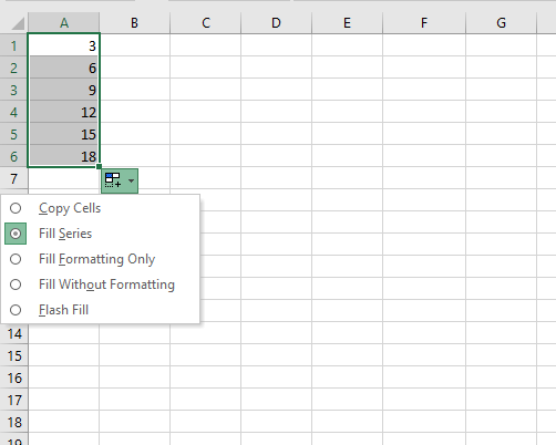
So if Excel completed a series based on a pattern it picked up, but what you actually wanted was to replicate the existing values, you’d select “Copy Cells.”

AutoFill with series settings

There are all kinds of patterns when dates are involved. It could be daily, weekly, fortnightly - you get the picture. We can still get AutoFill to work for us when date patterns aren’t obvious, by using series settings.

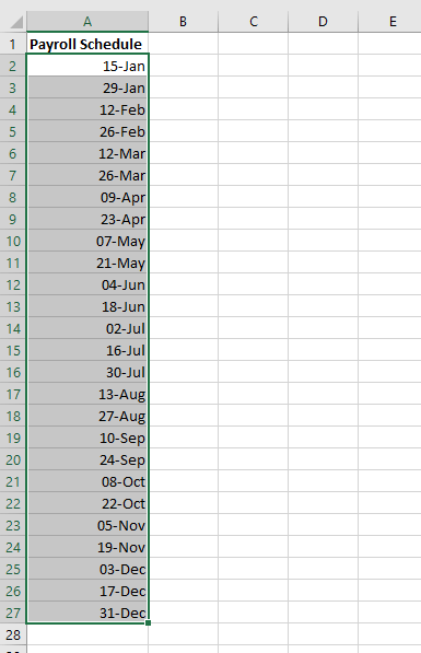
For instance, let's say we want to set up this year’s payroll schedule, which starts on January 15. We can activate a context menu by using the right mouse button when dragging along the range to be filled in.

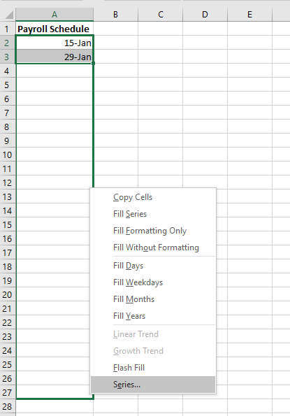
• Select “Series.” This opens the Series dialog box.
• The second column in the Series dialog box asks you to select the type of series represented by your dataset. Excel recognizes that our numbers are dates, but if your numbers aren’t so obvious, choose the right one.
• “Date unit”  wants you to choose which unit will be used to determine the next value. In our case, we select “Day.”
• The “Step Value” should be 14, since employees will get paid every 14 days.
• Click OK, and the Payroll Schedule is all filled in!

 

 

AutoFill using Custom Lists

What if your frequently-used list is something really unique which can’t be predicted by Excel, like the names of your team members, or the locations of your branches, or your product categories? These may be lists you need to enter over and over, and you probably wish there was a way you could quickly insert them when needed, instead of having to type them in one-by-one. Great news: there is.

To do this, you first need to create a Custom List. 

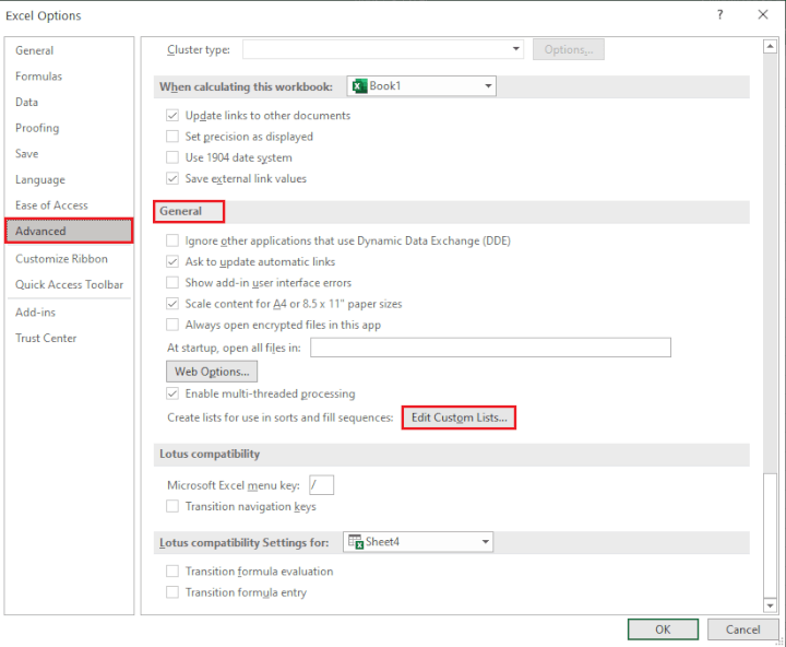
Create a Custom List in Windows operating systems:

• Click "File."
• Go to "Options."
• Select "Advanced."
• Click "Edit Custom Lists" in the “General” section.

 

• To the far left of the Custom Lists dialog box, Excel highlights the name “NEW LIST” for the list you are about to create. Enter the list items in the middle panel, using the Return or Enter key to separate items.
• Press Add, and your new list will be created below any existing custom lists.

 

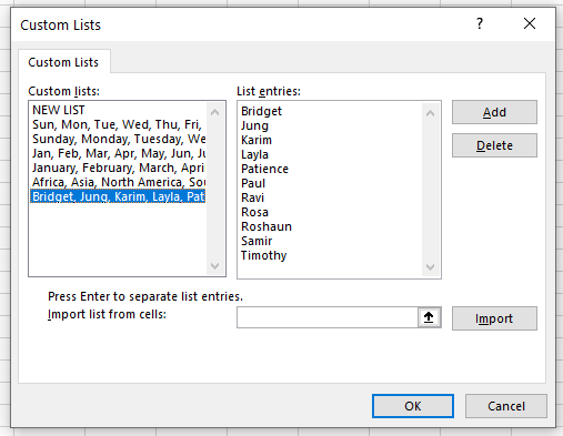
• Click OK.

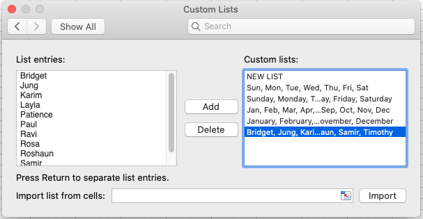
Create a custom list in Mac operating systems:

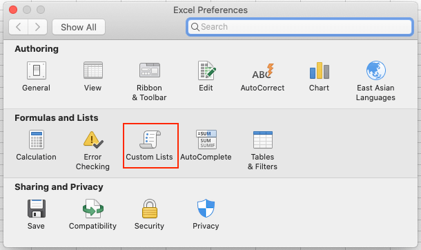
• Click Excel
• Go to Preferences
• Under “Formulas and Lists”, select Custom Lists

 

• This will open the Custom Lists dialog box. To the right, Excel highlights the name “NEW LIST” for the list you are about to create. Enter the list items in the left panel, using the return key to separate items
• Click Add, and your new list will be added to the available custom lists

 

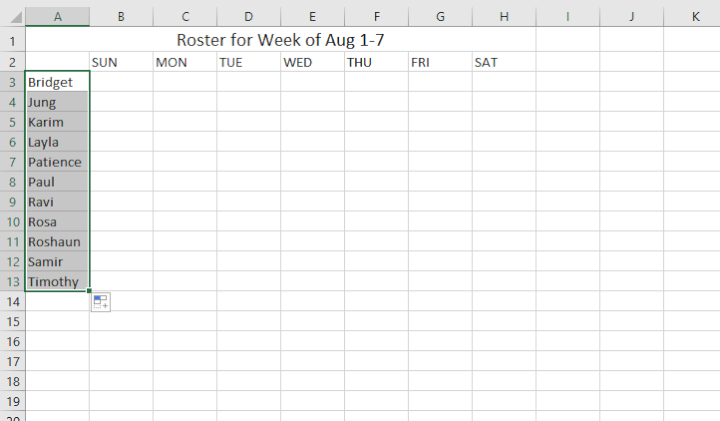
Your custom list is now ready to be used with AutoFill. Just type the first item, drag on the Fill Handle, and Excel will fill in the remaining items of your list.

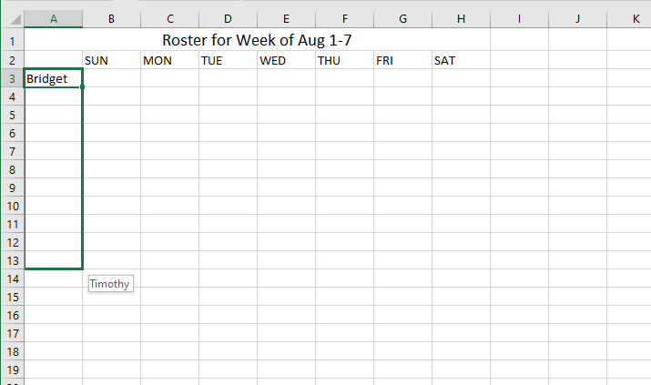
You can release when the last name is displayed.

Pretty cool, huh?

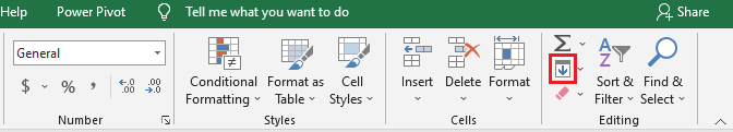
The Fill button on the Home tab

Here’s a little tip worth mentioning. You can also use the Fill command on the Home tab to do many of the tasks we’ve demonstrated above. 

But there is one innocent-looking option within that command which does something truly amazing.

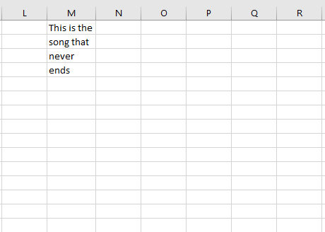
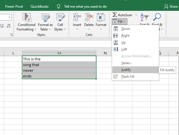
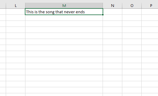
In the range below, we have text occupying four cells, which we would like to all be in a single cell. In other words, we’d like to merge or concatenate all these values. 

There are, in fact, several ways to do this in Excel, and the option chosen usually involves the use of a function, or at least the & operator.

Somewhat unexpectedly, the Fill button within the Editing group of the Home tab steps up here with a solution.

Here are the steps:

1. Expand the column so that it’s wide enough to accommodate the entire text. Otherwise, this method won’t work.
2. Highlight the entire range to be merged
3. Go to the Home tab > Editing command group > Fill command > Justify

Abracadabra!

Points to note when using the Fill > Justify command:

• You can’t merge numbers using this method. Fill > Justify works with text values only.
• You can merge up to 255 characters into a single cell. If you have more than 255 characters, the first 255 will be merged and the remaining characters will be distributed in the rows below.

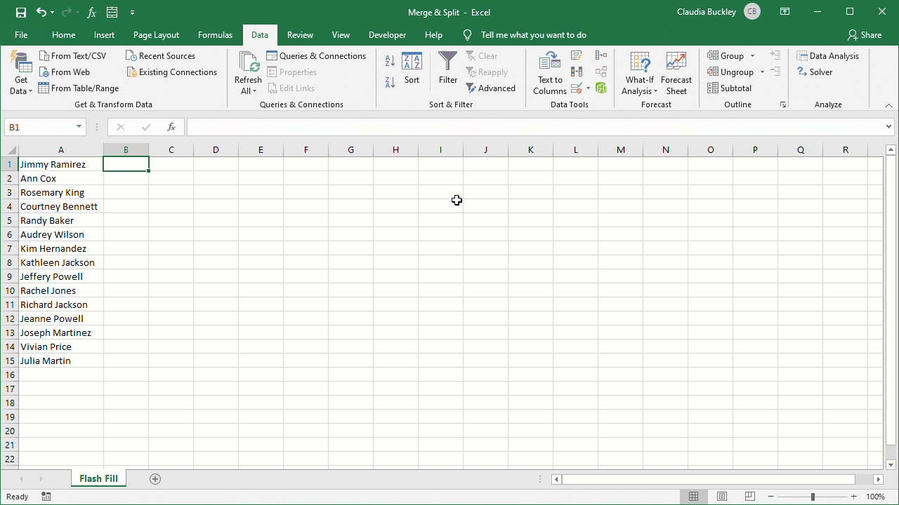
Flash Fill

We saved the best for last. As if everything we’ve seen so far wasn’t impressive enough, there’s Flash Fill.

If you need to convert data from one format to another, or extract certain values from a source dataset, you can teach Excel what you want your data to look like by entering the first two or three rows with the data in the desired format.

Next, click on the last value you entered, then click the Flash Fill icon from the Data tab in the Data Tools command group.

Repeat for each column, and voila! Your one-column data has been split across two columns.

In fact, sometimes Excel picks up on the pattern without you having to “teach” it. When Autofill thinks it found a pattern to flash fill, it will suggest that pattern by showing you a grayed-out version of what it thinks you want your completed data to look like. This is like the predictive text we commonly see in other kinds of technology. To accept, just hit the Tab key on your keyboard.

AutoComplete

Somewhat related to Autofill is AutoComplete. AutoComplete is a feature whereby Excel completes text entries that you start to type in a column of data if the first few letters entered match something you already entered in that column. Most times it’s useful, but AutoComplete can be disabled if you prefer.

You can disable AutoComplete by doing the following:

1. Click File > Options.

2. Click Advanced

3. Under Editing options, clear the Enable AutoComplete for cell values check box 

To re-enable AutoComplete, do Steps 1 and 2 above, then select the Enable Autocomplete for cell values check box under Editing Options.

More cool tricks

If you liked these time-saving tips, we think you’ll also like these 11 Excel Hacks You Need to Know Now. You’re welcome!

To learn more about Excel try our Excel - Basic and Advanced course today.

Level up your Excel skills

Become a certified Excel ninja with GoSkills bite-sized courses

Start free trial