How to Insert a Check Mark in Excel

---

Check marks have become a part of our task-oriented lives. If you use Excel to generate and execute lists (and you probably do), inserting an Excel checkmark symbol will come in mighty handy. In this tutorial, we’ll show you how to insert a check mark in Excel.

What is a check mark?

A check or tick mark (✓) is a symbol that is universally associated with a positive response (for example, yes, completed, correct, etc.). The tick symbol in Excel is treated as text. This means that the color and size can be changed like any other text would be, and the location can be changed using the standard Copy and Paste commands.

Check marks are not the same as check boxes. A check box in Excel is an object which is placed on a worksheet. A check box that appears to be in a cell will not be deleted if that cell is deleted, because the check box is not actually a part of the cell. The location of a check box can be changed by dragging it as you would any other object.

---

---

How to insert a check mark

There are multiple ways to insert a check mark in Excel. Five commonly-used methods are shown below.

Method 1: Shift P, Wingdings 2 font

A check mark is just another text character. If you can remember that SHIFT + P is that character, you can simply type an uppercase P in your desired cell, and change the font to Wingdings 2 as you would perform any regular font change. The Wingdings check mark will then be displayed in the worksheet.

You may also care to know that SHIFT + O in the Wingdings 2 font inserts the X symbol (×).

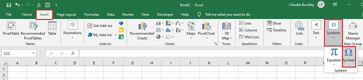
Method 2: Insert - symbol menu

The Excel ribbon has an Insert tab, and from there a Symbol dropdown. Choose the Symbol command and you will find all the supported symbols in Excel.  

In the Symbol dialog box, choose the Wingdings font option, and scroll down to find the check mark character. 

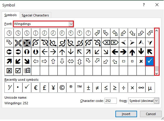Select the check mark and click the Insert button to place the check mark in the worksheet, then click Close to close the dialog window.

You can see in the above image that Excel stores recently used symbols toward the bottom of the Symbol dialog box to save time if you need to insert them again.

Method 3: ALT 0252

If you saw the character code 252 at the bottom of the dialog box in the previous method, this might be a good reminder of an Excel check mark shortcut.

You’ll need to change the font to Wingdings, then hold the ALT button while typing in 0252. Note that the numbers should be entered from the numeric pad on the keyboard, and not from the QWERTY numbers above the letters. 

If you forgot to change the font to Wingdings before doing the ALT 0252 shortcut, you may see a character that looks like this: ü. No worries. Just change that cell to the Wingdings font and your check mark will be displayed.

Note: There is no such option on Mac devices.

Method 4: UNICHAR function

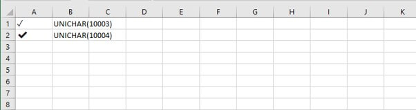
A check mark can be inserted using a function? Yes, it can. UNICHAR is a text function that returns the character represented by the Unicode argument in parentheses. Remember that each character is assigned a special code within the computer’s memory. Once you know the code for the character you want to insert, you can use UNICHAR to insert it.

=UNICHAR(10003) inserts a check mark, and UNICHAR(10004) inserts a heavy check mark.

This method offers the advantage of not having to change to a special font. If you choose to use the UNICHAR function, bear in mind that the check mark has to be the only value in that cell.

UNICHAR(10007) and UNICHAR(10008) will insert the X and heavy X, respectively.

Method 5: Conditional formatting

Conditional formatting tells cells how to behave if certain conditions are met. The Conditional Formatting feature can add icons into cells based on cell values, and you can use this feature to add a check mark in Excel.

---

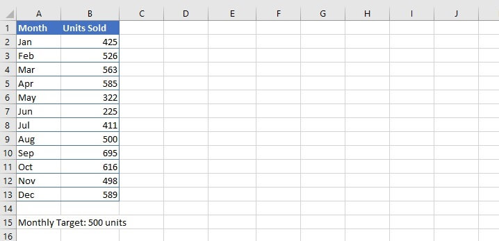
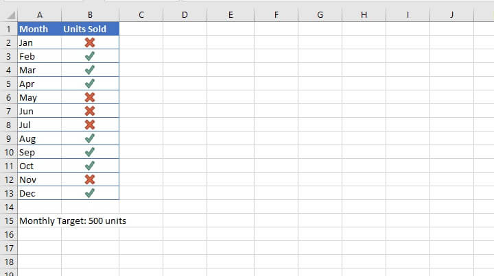
For example, download the practice file and work along while we use conditional formatting to insert a check mark next to each month where the target of 500 unit sales per month was met, and an X next to the months where the target was not met. 

---

To apply conditional formatting, follow the steps below:

1. Select the range where you want to place check marks (B2 to B13).
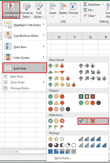
2. Go to the Home tab > click Conditional Formatting > then choose Icon Sets and select the set which includes the check mark indicator. This will be a 3-symbol icon set (a check mark, an X, and an exclamation mark). 

By default, Excel places a check mark for values within the 67th percentile and higher, and an X for values below the 33rd percentile. For values between the 33rd and 66th percentiles, an exclamation symbol is the default.

3. Change this default rule by going to the Manage Rules button under the Conditional Formatting menu while the data range is selected. This will bring up the Conditional Formatting Rules Manager window. Click the Edit Rules command to change the conditions under which these symbols are applied.
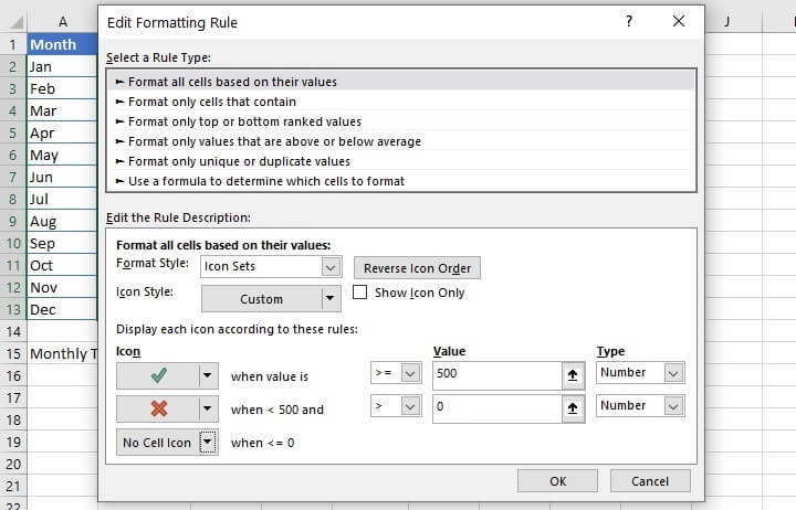
4. In the lower third of the Edit Formatting Rule window, change Percent to Number under the Type dropdown, and change the value 67 to 500. This will cause cells that are greater than or equal to 500 to have a check mark inserted.
5. Just below that, change the exclamation symbol to an X from the Icon dropdown, change the >= symbol to >, the Type to Number, and the Value to 0.
6. For the third symbol, click the dropdown and select No cell icon.

7. Click OK to confirm your changes and OK to apply them and return to the worksheet.

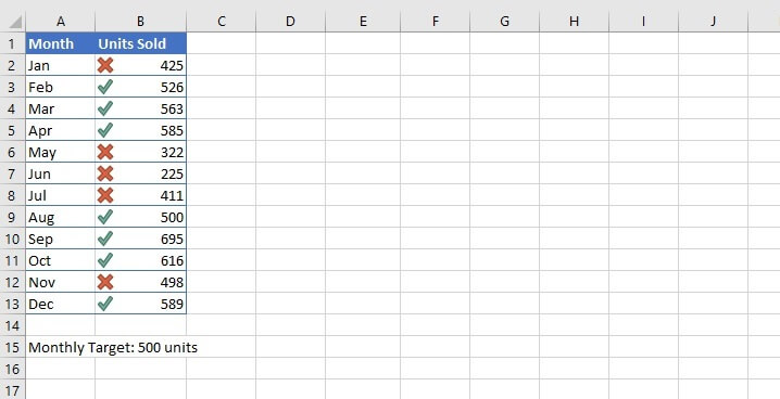You will now be able to tell at a glance whether the monthly target was met or not.

There is also the option of displaying the symbols only, without the associated number. Do this by returning to the Conditional Formatting Rules Manager, choosing Edit Rule, and then selecting the Show Icon Only checkbox.

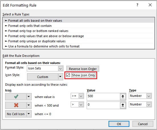When applied, the cells will now display the icons only.

Of course, since the check mark behaves just like a text character, you can make it bold, color it, increase the font size, change the alignment, and apply any other text formatting you like.

Learn more

Easy breezy. If you’ll be using check marks in Excel often, decide on your one or two favorite methods and practice them. 

Like what you learned? Try the GoSkills range of Excel courses to see what else you can learn in Excel. You can try our Microsoft Excel - Basic and Advanced course. Or start with our free Excel in an Hour course to learn some basics in Excel.

Learn Excel for free

Start learning formulas, functions, and time-saving hacks today with this free course!

Start free course