
Microsoft Excel is an immensely powerful tool, brimming with features that can turn the laborious task of sifting through data into an efficient and accurate process. One set of features, commonly used but not always understood, is the “IF family” of functions. This article is a beginner’s guide to understanding the purpose, logic, and real-world examples of Excel's IF functions.
What are IF functions in Excel?
IF functions are practical tools in Excel that enable us to automate decisions in our spreadsheets by using logical testing. They serve as inbuilt 'decision-making' aids for Excel, allowing data analysis based on set conditions.
Why use IF functions?
Simply put, IF functions help automate your Excel tasks. Whether it's grading students' tests based on their scores, counting the number of sales reps who met their targets, or deciding if a loan application should be approved based on certain financial ratios, the IF function can do these tasks efficiently, accurately, and most importantly, automatically.
Get your FREE cheatsheet!
Download your printable cheatsheet with the top 10 Excel IF functions.
Top 10 IF statements in Excel
1. IF
=IF(logical_test, [value_if_true], [value_if_false])| What it does | Returns one value if a statement is true, and another value if it is false. |
|---|---|
| Syntax | IF(logical_test, [value_if_true], [value_if_false]) |
| What the arguments mean |
logical_test is the statement to be tested. value_if_true is what to do if the statement is true*. value_if_false is what to do if the statement is false*. |
| Remarks |
Logical tests are used with logical operators (>, <, =). * At least one of the two optional arguments must be provided so that Excel knows what to do. |
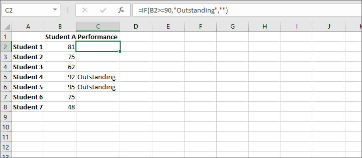
| How to use IF in Excel | =IF(A2>=90, "Outstanding", "") will display the text "Outstanding" if the value in cell A2 is greater than or equal to 90. Otherwise, a blank will be displayed. |
2. IFS
=IFS(logical_test1, value_if_true1, [logical_test2, value_if_true2],...)| What it does | Returns values based on the outcome of two or more logical tests. Use this function when you have more than two possible outcomes. |
|---|---|
| Syntax | IFS(logical_test1, value_if_true1, [logical_test2, value_if_true2],...) |
| What the arguments mean |
logical_test1 is the formula or expression to be evaluated. value_if_true1 is the value to return if logical_test1 is true. logical_test2 and subsequent, are additional formulas or expressions to be evaluated (optional). value_if_false2 and subsequent, are the values to return if the matching logical tests are true. |
| Remarks |
Conditions are applied in the order in which they appear in the formula. If a condition is found to be TRUE, Excel returns the associated value_if_true without evaluating the remaining tests. Unlike the IF function, there is no “value_if_false” argument in the IFS function. The logical expression TRUE can be used as a logical test to return the desired value_if_false. Up to 127 tests are permitted. Available in Excel 2019 and later. |
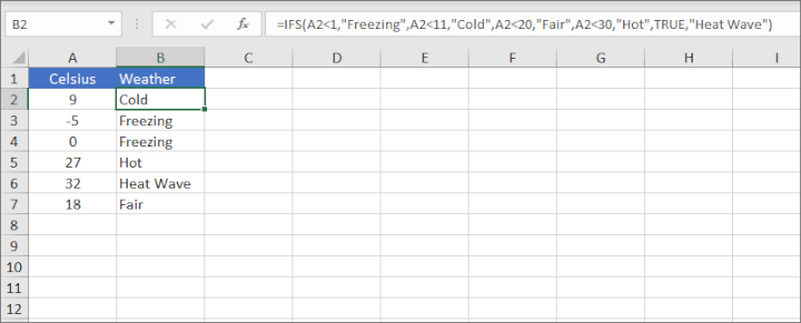
| How to use IFS in Excel | See example below. |
3. AVERAGEIF
=AVERAGEIF(range, criteria, [average_range])| What it does | Returns the average (arithmetic mean) of all the cells in a range that meet a certain condition. |
|---|---|
| Syntax | AVERAGEIF(range, criteria, [average_range]) |
| What the arguments mean |
range is the group of cells to be evaluated. criteria is the value or expression in range to search for. average_range (optional) is the range of cells to be averaged. If omitted, the cells in range are used. |
| Remarks |
Empty criteria cells are given a value of zero. Empty average_if cells are ignored. If no cells in the range meet the criteria, AVERAGEIF returns the #DIV/0! error value. Wildcard characters (*, ?, ~) are supported for partial matches. To average cells based on multiple criteria, use the AVERAGEIFS function instead. |
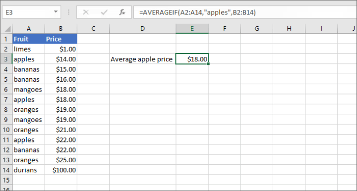
| How to use AVERAGEIF in Excel | See example below. |
4. AVERAGEIFS
=AVERAGEIFS(average_range, criteria_range1, criteria1, [criteria_range2, criteria2], ...)| What it does | Returns the average (arithmetic mean) of cells that meet multiple criteria. |
|---|---|
| Syntax | AVERAGEIFS(average_range, criteria_range1, criteria1, [criteria_range2, criteria2], ...) |
| What the arguments mean |
average_range is the group of cells to be averaged. criteria_range1 is the range where the first criteria may be found. criteria1 is the criteria to look for in criteria_range1. criteria_range2 (optional) is the range of cells to be averaged. If omitted, the cells in range are used. |
| Remarks |
AVERAGEIFS evaluates cells across the entire row. If a cell in a criteria range fails to meet its corresponding criteria, that row is eliminated from being averaged. To find the average of cells that meet any of the stated criteria, the AVERAGEIF function should be nested into the AVERAGE function. Available in Excel 2019 and later. |
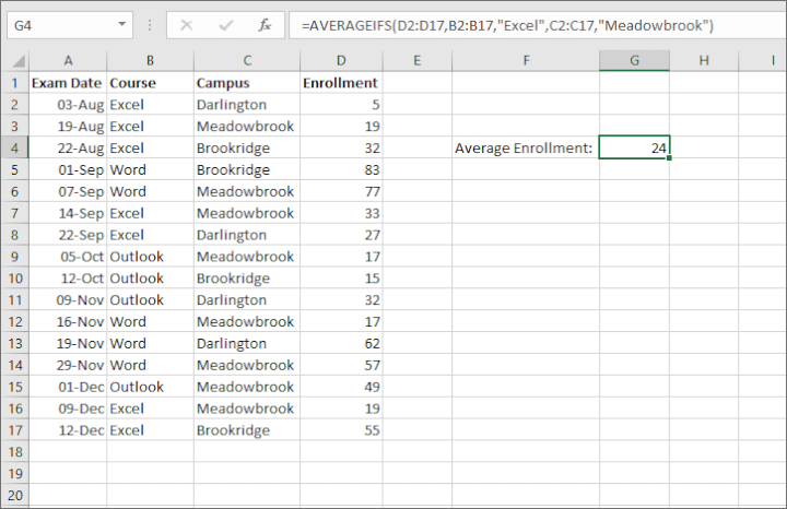
| How to use AVERAGEIFS in Excel | See example below. The formula below calculates the average number of enrollments for Excel at the Meadowbrook campus. |
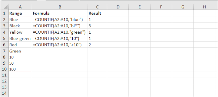
5. COUNTIF
=COUNTIF(range, criteria)| What it does | Counts the number of cells within a range meet a given criteria. |
|---|---|
| Syntax | COUNTIF(range, criteria) |
| What the arguments mean |
range is the range of cells to be evaluated. criteria is the value or expression to search for. |
| Remarks |
When the criterion is entered in the form of a cell reference, no double quotes are used. In the COUNTIF default setting, cell contents must be an exact match to be counted. Wildcard characters (*, ?, ~) are supported for partial matches. COUNTIF is not case-sensitive. |
| How to use COUNTIF in Excel | See example below. |
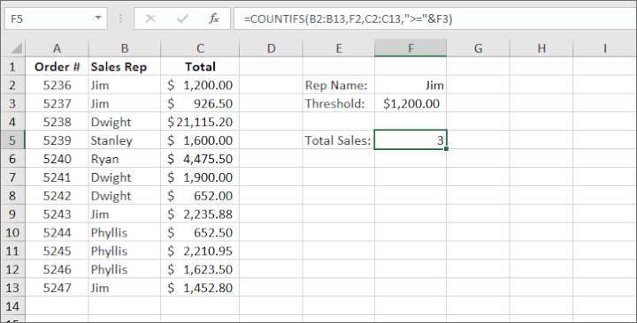
6. COUNTIFS
=COUNTIFS(criteria_range1, criteria1, [criteria_range2, criteria2…])| What it does | Counts the number of cells within a range that meet multiple criteria. |
|---|---|
| Syntax | COUNTIFS(criteria_range1, criteria1, [criteria_range2, criteria2…]) |
| What the arguments mean |
criteria_range1 is the first range of cells to be evaluated. criteria1 is the value or expression in criteria_range1 to search for. criteria_range2, criteria2 and all subsequent argument pairs are optional. |
| Remarks |
All criteria_ranges must be the same dimensions. COUNTIFS evaluates each range for its criteria individually, but each corresponding row must satisfy all conditions in order to be counted. Available in Excel 2019 and later. |
| How to use COUNTIFS in Excel | See example below. The formula only counts the number of sales made by Jim where the value was greater than or equal to $1200. |
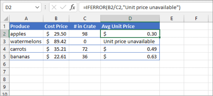
7. IFERROR
=IFERROR(value, value_if_error)| What it does | Performs specified action if a formula results in an error. |
|---|---|
| Syntax | IFERROR(value, value_if_error) |
| What the arguments mean |
value is the formula or expression that is checked for an error. value_if_error is the value to return if value results in an error. |
| Remarks |
IFERROR considers the following results as errors: #N/A, #VALUE!, #REF!, #DIV/0!, #NUM!, #NAME?, #NULL! If value does not result in an error, Excel returns the result of value. |
| How to use IFERROR in Excel | =IFERROR(100/0,”Invalid result”) returns Invalid result. |
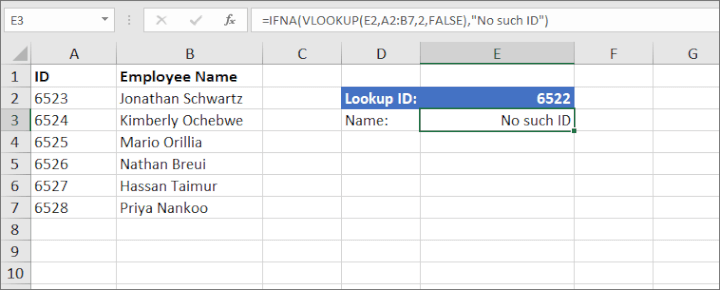
8. IFNA
=IFNA(value, value_if_na)| What it does | Performs specified action if a formula results in the #N/A error. |
|---|---|
| Syntax | IFNA(value, value_if_na) |
| What the arguments mean |
value is the formula or expression that is checked for an error. value_if_na is the value to return if value results in an #N/A error. |
| Remarks |
#N/A errors are usually the result of a failed lookup value. If value does not result in an #N/A error, Excel returns the result of value. |
| How to use IFNA in Excel | See example below. |
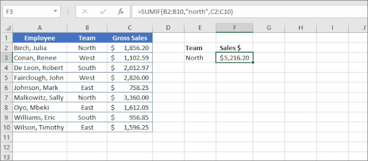
9. SUMIF
=SUMIF(range, criteria, [sum_range])| What it does | Finds the sum of cells within a range that meet a given criterion. |
|---|---|
| Syntax | SUMIF(range, criteria, [sum_range]) |
| What the arguments mean |
range is the group of cells to be evaluated. criteria is the value or expression in range to search for. sum_range (optional) is the range of cells to be summed. If omitted, the cells in range are summed. |
| Remarks |
When the criterion is entered in the form of a cell reference, no double quotes are used. In the SUMIF default setting, cell contents must be an exact match to be counted. Wildcard characters (*, ?, ~) are supported for partial matches. SUMIF is not case-sensitive. Range and sum_range (if used) must be the same dimensions for accuracy. To sum cells based on multiple criteria, use the SUMIFS function instead. |
| How to use SUMIF in Excel | See example below. |
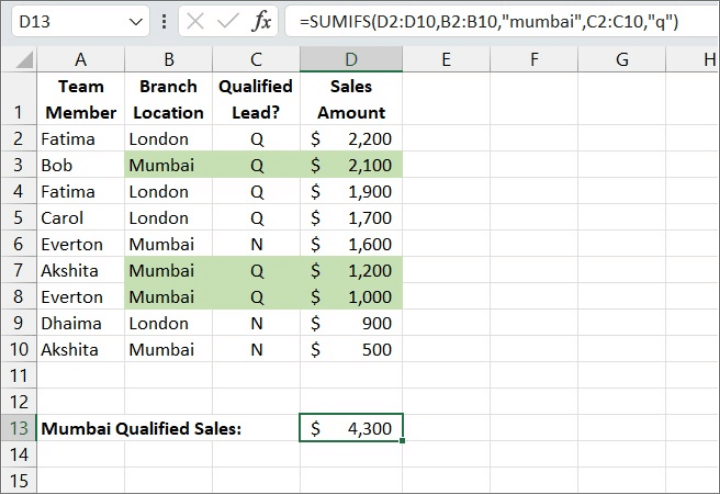
10. SUMIFS
=SUMIFS(sum_range, criteria_range1, criteria1, [criteria_range2], [criteria2]...)
| What it does | Finds the sum of cells within a range that meet all the stated criteria. |
|---|---|
| Syntax | SUMIFS(sum_range, criteria_range1, criteria1, [criteria_range2], [criteria2]...) |
| What the arguments mean |
sum_range is the range of cells to be summed. criteria_range1 is the first range of cells to evaluate for the presence of the criteria1. criteria1 is the condition associated with criteria_range1 which must be satisfied for the corresponding value in sum_range to be added. |
| Remarks |
SUMIFS looks at each criteria range for its associated criterion. For example, criteria1 is associated with criteria_range1. Criteria2 is associated with criteria_range2 and so on. Up to 127 pairs of criteria may be entered. SUMIFS will return a #VALUE error if the ranges are not the same size. Wildcard characters (*, ?, ~) are supported for partial matches. Available in Excel 2019 and later. |
| How to use SUMIFS in Excel | See example below. |
 Note on SUMIFS ranges: SUMIFS determines matches by looking at each criterion’s position with its respective range, therefore SUMIFS may be used on ranges that start and end on different rows, but must be of the same dimension. If the corresponding position in each range matches the position number of the other ranges, then that sum_range position is counted.
Get your FREE cheatsheet!
Download your printable cheatsheet with the top 10 Excel IF functions.
Parting words
Excel IF functions empower us to apply logical decision-making within our spreadsheets, improving efficiency and productivity. These functions, with their conditional logic, help us operate sophisticated data manipulation with minimal human intervention. Once you start using IF functions, they will inevitably become a crucial part of your Excel toolkit, handling much of the heavy lifting that data management requires. Remember, Excel isn't just a spreadsheet tool. It's a powerful assistant that can simplify and automate your tasks if you know how to make good use of its features.
A structured course that allows you to learn at your own pace is the best way to learn the skills you need while getting as much practice as you want. Choose the Excel course that’s right for you from our regularly updated course library.