How to use TEXTBEFORE, TEXTAFTER and TEXTSPLIT in Excel

In the first quarter of 2022, Microsoft announced 14 new Excel functions that make working with text operations and transforming arrays much easier than before.

Below, we’ll share examples of how to use the required and optional arguments for the ones specifically designed to parse text - TEXTBEFORE, TEXTAFTER, and TEXTSPLIT. 

Availability

If you want to practice and find that you don’t have these 14 new text and array functions, it’s likely that they aren’t available because you don’t have a current Microsoft 365 subscription. Don’t worry, you can still access them using Excel Online for free.

Split text strings

TEXTBEFORE, TEXTAFTER, and TEXTSPLIT are designed for text manipulation and will eventually become the preferred option instead of having to combine the LEFT, RIGHT, or MID functions with SEARCH, FIND, SUBSTITUTE, or REPLACE.

 

TEXTBEFORE

Purpose

Returns all text that occurs before (to the left of) a specific character, or delimiter. 

Syntax

=TEXTBEFORE(text, delimiter, [instance_num], [ignore_case])

Arguments

text	This is the text or cell reference containing text you will be working with.
delimiter	All text before this character will be extracted.
instance_num (optional)	This argument determines which occurrence of the delimiter should be used. The default instance_num is 1 (meaning the first observed instance of the delimiter).
ignore_case (optional)	TRUE will search for uppercase and lowercase instances of the delimiter. FALSE will search for the delimiter in the case used in the delimiter argument. The default is FALSE.

Remarks

1. Wildcard characters are not allowed.
2. If the delimiter is not found within the text string, Excel returns a #VALUE! error.

In the examples below, we will compare the advantages of TEXTBEFORE.

TEXTBEFORE vs. LEFT function

While LEFT will continue to remain useful for splitting text after a fixed number of characters, TEXTBEFORE will replace many of the combinations we previously used to split text using a specific character (delimiter) to mark the separation point.

Split text strings of variable length

Of course, when the number of characters is known and fixed (for example, phone numbers), using the LEFT function to split text is no problem. Text strings of varying lengths, however, mean that we have to find a way to determine where one column ends and the new one begins (the num_chars argument). This was previously accomplished by combining LEFT with the SEARCH or FIND functions to locate the appropriate delimiter.

=LEFT(A2,SEARCH(",",A2)-1)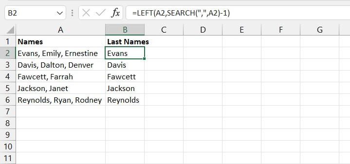

Of course, the above formula works well when nesting principles are understood, but is sometimes intimidating to beginners or casual Excel users.

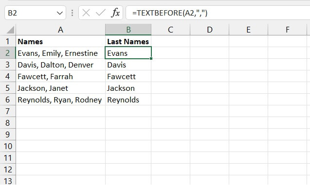
With TEXTBEFORE we can easily extract the last names from column A by using the first comma (placed within double quotes) as the delimiter. Since TEXTBEFORE defaults to the first instance of the delimiter, we only need the required arguments.

=TEXTBEFORE(A2,”,”)

Extract substring with case-sensitive option

In the following example, we can extract the username portion of the email addresses ending in “@xyz.net” by combining LEFT with the FIND function. 

=LEFT(A2,FIND(“@xyz.net”,A2)-1)

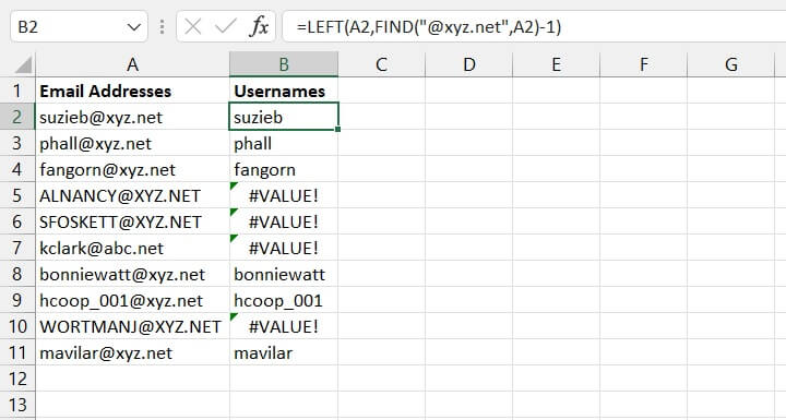
The FIND function is case sensitive, so the uppercase “XYZ.NET” values are not considered matches and return a #VALUE! error. The user would have had to use the SEARCH function instead of FIND to perform a case-insensitive search. 

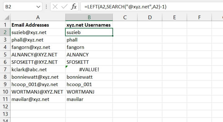
=LEFT(A2,SEARCH("@xyz.net",A2)-1)

TEXTBEFORE gives the option of switching case sensitivity on and off. This not only relieves you from having to remember whether SEARCH or FIND is case sensitive, but also from having to combine functions in the first place.

To make the delimiter case sensitive, we can either omit the ignore_case argument or choose FALSE.

=TEXTBEFORE(A2,"@xyz.net",,FALSE)

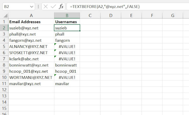
Note that the instance_num argument is skipped by simply typing a comma to move on to the next argument.

=TEXTBEFORE(A2,"@xyz.net")

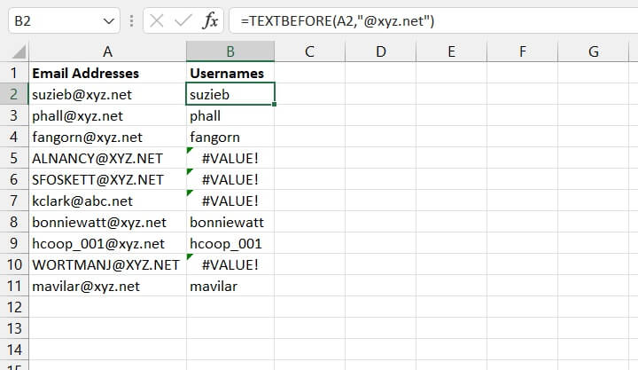
The result is the same. 

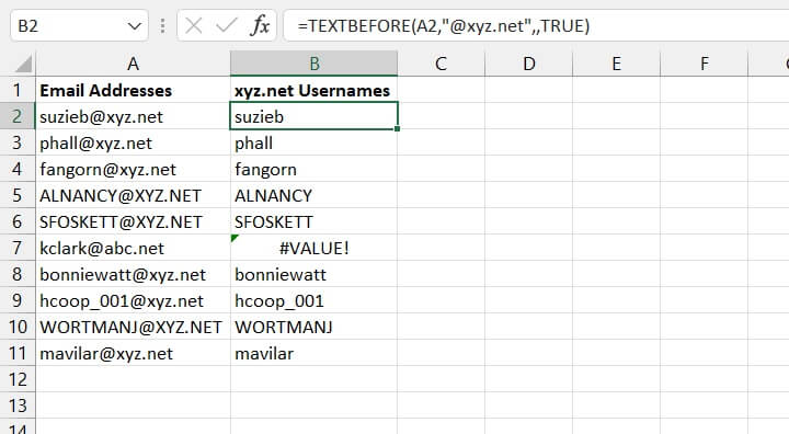
To return all “@xyz.net” usernames, regardless of the case, we would enter TRUE for the ignore_case argument.

=TEXTBEFORE(A2,”@xyz.net”,,TRUE)

Note - To prevent Excel from displaying errors, consider using the IFERROR function.

TEXTAFTER

Purpose

Returns all text that occurs after (to the right of) a specific character, or delimiter. 

Syntax

=TEXTAFTER(text, delimiter, [instance_num], [ignore_case])

Arguments

text	This is the text or cell reference containing text you will be working with.
delimiter	All text after this character will be extracted.
instance_num (optional)	This argument determines which occurrence of the delimiter should be used. The default instance_num is 1.
ignore_case (optional)	TRUE will search for uppercase or lowercase delimiter. FALSE will search for the delimiter in the case used. The default is FALSE.

Remarks

1. Wildcard characters are not allowed.
2. If the delimiter is not found within the text string, Excel returns a #VALUE! error.

TEXTAFTER vs. RIGHT function

Since TEXTAFTER extracts text after a given delimiter, it can be compared to the RIGHT function, which splits text toward the end of a text string.

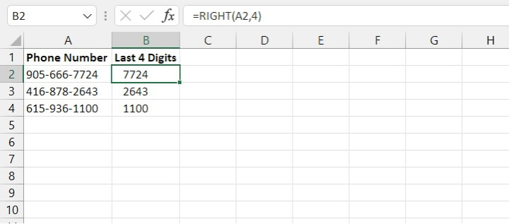
The RIGHT function works well when we know exactly how many characters we want to extract. For example, we would get the last four digits of a phone number with the entry:

=RIGHT(A2,4)

 

But when the length of the text string is unknown, we have had to find creative ways of determining where the substring ends.

=RIGHT(A2,LEN(A2)-SEARCH(", ",A2)-1)

 

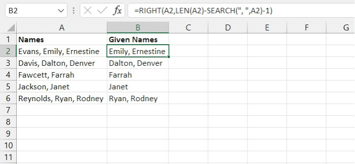
The above formula searches for the first occurrence of the delimiter and subtracts that position number from the length of the entire string. It is then embedded (nested) within the RIGHT function to extract the text that comes after the delimiter.

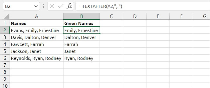
With TEXTAFTER, the formula would simply be:

=TEXTAFTER(A2,", ")

The instance_num and ignore_case arguments in TEXTAFTER work in the same way as explained in TEXTBEFORE.

TEXTSPLIT

Purpose

Splits text into columns or rows based on a specified delimiter.

Syntax

=TEXTAFTER(text, col_delimiter, [row_delimiter], [ignore_empty], [pad_with])

Arguments

text	This is the text or cell reference containing text you will be working with.
col_delimiter	This character will be treated as the column separator.
row_delimiter (optional)	This character will be treated as the row separator.
ignore_empty (optional)	TRUE will display empty cells when Excel encounters consecutive delimiters within the original string. The default is FALSE (will not display empty cells).
pad_with (optional)	This text will be used to fill out missing values in a 2D array. The default is #N/A.

Remarks

1. Col_delimiter is optional when row_delimiter is present and vice versa.
2. TEXTSPLIT results in a spilled array. Therefore, all cells where the results will be returned must be empty. Otherwise, Excel will return a #SPILL! error. 

TEXTSPLIT vs. Text to Columns

The Text to Columns command is a built-in tool to convert a single column of text into multiple columns.

The TEXTSPLIT function is an improvement over Text to Columns because it is dynamic, that is, the results automatically update when the source data changes. This behavior is another inherent feature of Microsoft 365’s dynamic arrays.

TEXTSPLIT vs. LEFT, RIGHT, MID

The most obvious advantage of the TEXTSPLIT function is its efficiency, as shown in the following examples. 

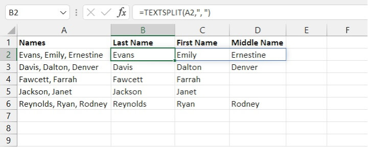
Instantly split text into separate columns

One function can now split the values in a cell into different columns – a task that previously took at least three functions and three different entries. Since the results of TEXTSPLIT automatically spill as a feature of dynamic arrays, there is no need to split each one individually.

=TEXTSPLIT(A2,", ")

TEXTSPLIT vs. Power Query to separate text into rows

With the help of Power Query, we can not only split text into columns but rows too. Though this is relatively straightforward, many people are still intimidated by Power Query.

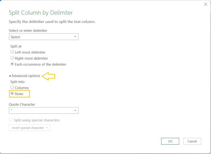
The TEXTSPLIT alternative allows text strings to be split into columns, rows, or both using a worksheet function.

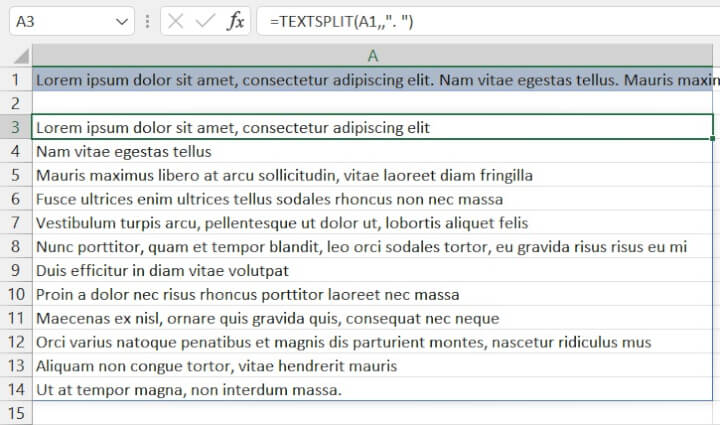
In the example below, we will place each sentence in a new row using TEXTSPLIT.

=TEXTSPLIT(A1,,". ")

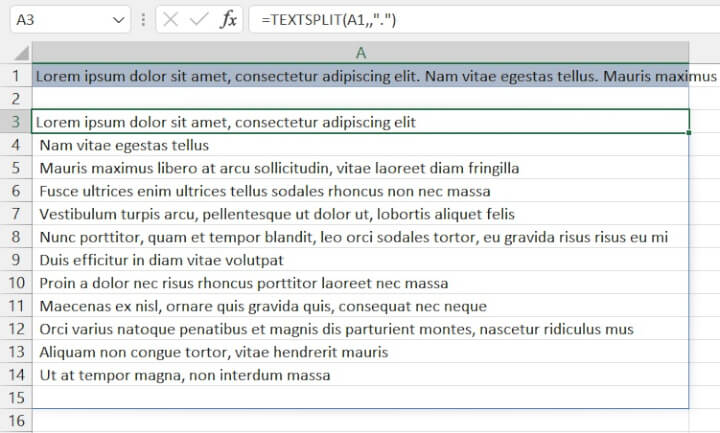
Note that the col_delimiter argument is skipped since a row_delimiter is provided.

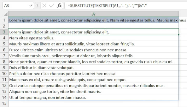
If we wanted to reintroduce periods at the end of each sentence without duplicating the final period, we would use the SUBSTITUTE function to remove the final period and simply use one of the concatenation methods to add them back to each row.

=SUBSTITUTE(TEXTSPLIT(A1,,". "),".","")&"."

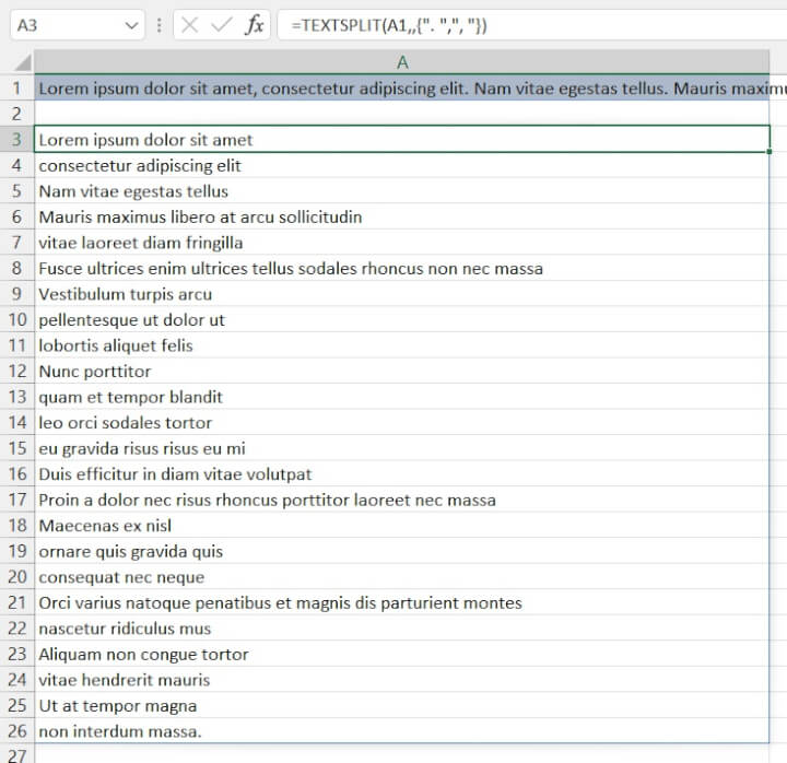
Multiple delimiters to split text

For situations where there may be multiple delimiters, an array constant in the format {“a”, “b”} can be used for the respective TEXTSPLIT delimiter argument.

In the following example, the values in cell A1 are split into different rows whenever Excel encounters a “period-space” or “comma-space”. 

=TEXTSPLIT(A1,,{". ",", "})

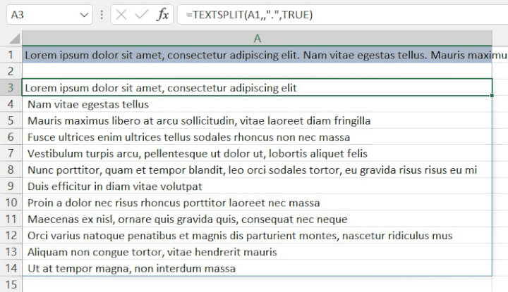
Suppress empty rows or columns

Sometimes TEXTSPLIT returns an empty row or column because two delimiters appear together, or a delimiter appears at the end of the text string. Below, the row_delimiter is a period, so an empty row was created below cell A14.

=TEXTSPLIT(A1,,".")

The ignore_empty argument can be set to TRUE as shown below to suppress the empty row.

=TEXTSPLIT(A1,,".",TRUE)

Two-dimensional arrays

Our final example shows how the pad_with argument works. When TEXTSPLIT returns a two-dimensional array, some rows or columns will likely have fewer values than others. 

Pad_with is an optional argument that tells Excel how to handle empty cells at the end of the shorter rows. If the pad_with argument is omitted, those cells will display an #NA error.

=TEXTSPLIT(A1," ",". ")

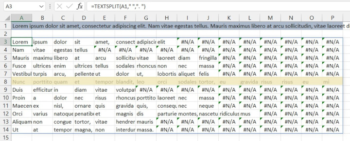
As shown above, row 8 returns values all the way to column P. The other rows return an #N/A error in the cells of the spill range that have no values. To display an alternative result, enter a pad_with value as text within double quotes, or by using a cell reference.

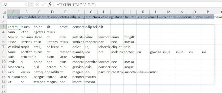
For example, to display an empty cell, the formula would be:

=TEXTSPLIT(A1," ",". ",,"")

Summary

Since splitting values into separate columns and rows is usually just a first step before doing a deeper dive into data analysis, it’s a breath of fresh air that these tasks can now be done natively with ease.  You can also learn how to use Excel TEXTJOIN to join multiple strings into one.

Here are the key takeaways from this article:

• The TEXTBEFORE, TEXTAFTER, and TEXTSPLIT functions are designed for text manipulation and will replace many of the previously used combinations of functions.
• TEXTBEFORE extracts all text that occurs before a specific character or delimiter, and it can be case-sensitive or case-insensitive.
• TEXTAFTER extracts all text that occurs after a specific character or delimiter.
• TEXTSPLIT splits text into columns or rows based on a specified delimiter, and it is more dynamic and efficient than the built-in Text to Columns command.
• TEXTSPLIT also allows text strings to be split into columns, rows, or both using a worksheet function.
• These functions make splitting values into separate columns and rows much easier, which is usually a first step before doing a deeper dive into data analysis.

If you want to learn more about how to use Microsoft Excel and become proficient at data analysis, check out this free course to help you master Microsoft Excel.

Ready to become a certified Excel ninja?

Start learning for free with GoSkills courses

Start free trial