Top 12 Excel Lookup Functions (+ Free Cheatsheet!)

Excel can perform a wide range of operations. The day I used my first VLOOKUP formula was the day I knew my Excel spreadsheets were more than just a handy place to store data. 

Whether you're a beginner or an experienced user, understanding the various functions you can use to look for values within a specified range of cells or to locate characters within a single cell can greatly enhance your productivity and make you indispensable among your colleagues. And we’re not just talking about Ctrl+F to find and replace values. 

The following functions are for when you have lots of data but you only want to look up, extract, and/or work with a portion of that data. From simple lookups to complex data extraction, these functions will empower you to make the most of Excel's capabilities and streamline your data analysis processes.

In this article, I’ll share my top 12 functions to look up or extract data in Excel and how to use them. This will equip you with the expertise to efficiently retrieve and manipulate vital information within your spreadsheets. 

Best of all, you can download and print the cheat sheet below and keep it for easy reference.

 1. VLOOKUP function

What does VLOOKUP do in Excel?

VLOOKUP is the Excel function that changed everything. It searches for a value in the first column of an array and returns the corresponding value from the nth column when a match is found.

The format of the VLOOKUP  function is as follows:

=VLOOKUP(lookup_value, table_array, col_index_num, [range_lookup])

VLOOKUP function: What do the arguments mean?

• lookup_value is the value you are looking for.
• table_array is the table array or database to be searched.
• col_index_num is the column number where possible return values are located.
• range_lookup (optional) is a setting to force an exact match or to accept approximate matches when no exact match is found. If omitted, approximate matches are allowed.

How to use VLOOKUP in Excel

Example 1: VLOOKUP with exact match

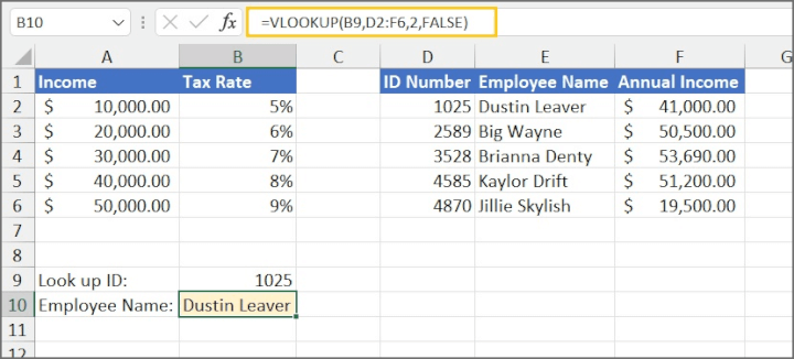Explanation: In this example, we are using the employee ID as the lookup value within the dataset D2:F6. The value we want to return will be from column 2 of the array, and we need an exact match, so the final argument is FALSE.

The value is found in cell D2. Therefore, the return value is “Dustin Leaver”.

Example 2: VLOOKUP with approximate match

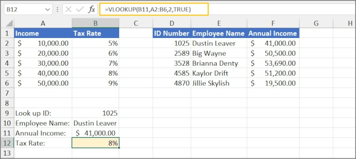Explanation:  In this example, we are using the employee’s annual income as the lookup value within the dataset A2:B6. The value we want to return will be from column 2 of the array. Since the incomes in column A are thresholds and may not be the exact amount of the employee’s annual income, we want Excel to use an approximate match if no exact match is found. Therefore, the final argument is TRUE.

$41,000 is not found in the array, and since that value falls between $40,000 and $50,000, Excel will treat the smaller value as its approximate match. The tax rate for $41,000 is thus 8%.

Important notes about the VLOOKUP function

• The column containing lookup_values must be located in the first column of the table_array.
• For the approximate match setting to work correctly, lookup_values must be sorted in ascending order.
• When range_lookup = FALSE, an #N/A error is returned if no exact match is found.
• If you have Microsoft 365 or later, consider using XLOOKUP instead, as it is simpler to use and offers more flexibility than VLOOKUP.

2. HLOOKUP function

What does HLOOKUP do in Excel?

HLOOKUP is the horizontal version of VLOOKUP. It searches for a value in the first row of an array and returns the corresponding value from the nth row when a match is found.

The format of HLOOKUP is as follows:

=HLOOKUP(lookup_value, table_array, row_index_num, [range_lookup])

HLOOKUP function: What do the arguments mean?

• lookup_value is the value you are looking for.
• table_array is the table array or database to be searched.
• row_index_num is the row number where the possible return values are located.
• range_lookup (optional) is a setting to force an exact match or to accept approximate matches when no exact match is found. If omitted, approximate matches are allowed.

How to use HLOOKUP in Excel

Example 1: HLOOKUP with exact match

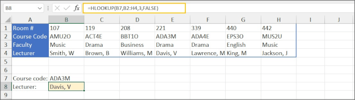
=HLOOKUP(B7,B2:H4,3,FALSE)

In this example, we are searching for the value in cell B7 within the array B2:H4. If the value is found, we expect Excel to return the corresponding value from the second row of the array. We are only looking for an exact match.

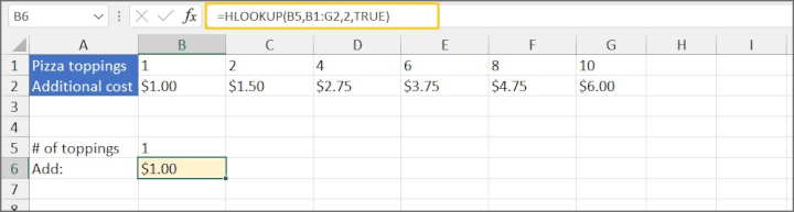
Example 2: HLOOKUP with approximate match

Important notes about the HLOOKUP function

• The row containing lookup_values must be located in the first row of the table_array.
• For the approximate match setting to work correctly, lookup_values must be sorted in ascending order from left to right.
• When range_lookup = FALSE, an #N/A error is returned if no exact match is found.
• If you have Microsoft 365 or later, consider using XLOOKUP instead as it is simpler to use and offers more flexibility than HLOOKUP.

3. XLOOKUP function

What does XLOOKUP do in Excel?

XLOOKUP is considered an upgraded version of VLOOKUP. It searches a range or an array, and returns the corresponding item when a match is found, but importantly, it is flexible enough to search horizontally, vertically, to the left, or right. Therefore, unlike VLOOKUP and HLOOKUP, the lookup values can be in any position relative to the return values.

The format of XLOOKUP is as follows:

=XLOOKUP(lookup_value, lookup_array, return_array, [if_not_found], [match_mode], [search_mode])

XLOOKUP in Excel: What do the arguments mean?

• lookup_value is the value used to do the search.
• lookup_array is the range or array where the lookup values may be found.
• return_array is the range or array containing potential return values.
• if_not_found (optional) is the text to display if no match is found.
• match_mode (optional) is a setting to force Excel to look for an exact match to the lookup_value, to accept approximate matches if no exact match is found, or to search with wildcard characters. If omitted, Excel looks for an exact match.
  • 0:  exact match
  • -1: closest smaller match if exact match not found
  • 1:  closest larger match if exact match not found
  • 2:  wildcard character match
• search_mode (optional) is a setting to search from first to last or reverse order, or to perform a binary search. If this argument is omitted, XLOOKUP will perform a first-to-last search.
  • 1:  search first to last (top-to-bottom or left-to-right)
  • -1: search last to first (bottom-to-top or right-to-left)
  • 2:  binary search sorted in ascending order
  • -2: binary search sorted in descending order

How to use XLOOKUP in Excel

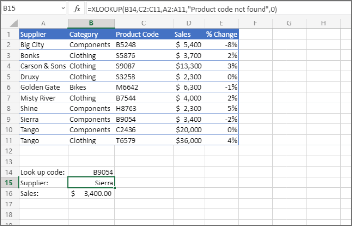
An XLOOKUP example with all arguments is shown below.

=XLOOKUP(B14, C2:C11, A2:A11, “Product code not found”,0)

The above formula is searching for the value in cell B14 within the range C2:C11. If the value is found, Excel should return the value in the corresponding row from the A2:A11 range. If the exact value is not found, the message, “Product code not found” will be displayed.

Important notes about the XLOOKUP function

• XLOOKUP is only available in Excel 365 or later.
• XLOOKUP can “spill” multiple return values if the columns or rows are adjacent.

Learn more about XLOOKUP here.

 4. FILTER function

What does FILTER do in Excel?

The Excel FILTER function extracts data from an array based on the conditions you specify and only returns rows that meet the stated criteria.

The format of the FILTER function is:

=FILTER(array, include, [if_empty])

FILTER in Excel: What do the arguments mean?

• array is the dataset containing the values you want to filter
• include is the specific range of cells containing the values to which the filter will be applies. This argument will also state the criteria.
• if_empty (optional) tells Excel what to do if there are no values that meet the condition stated in the include argument. If omitted, Excel will return a #CALC! error if the result is an empty array.

How to use the FILTER function in Excel

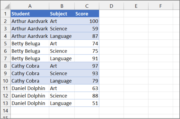
Some examples will be shown using the dataset below.

Example 1: FILTER with one criterion

=FILTER(A2:C13,B2:B13="Science")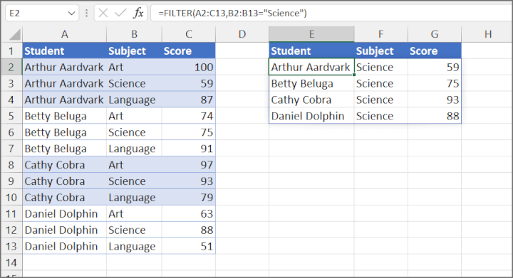

Explanation: The array is the original dataset containing all students’ scores. To isolate scores for Science, we specify in the include argument that values in the “Subject” column should be equal to “Science”.

Example 2: FILTER with multiple conditions (must satisfy at least one condition)

=FILTER(A2:C13,(B2:B13="Science")+(B2:B13="Art"))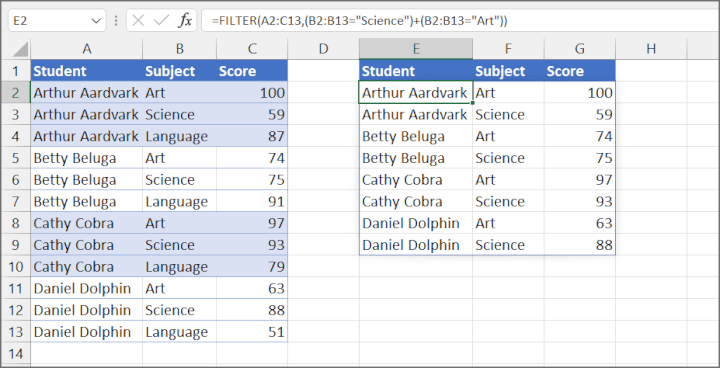

Explanation: The array is the original dataset containing all students’ scores. To lookup all student scores for Science and Art, we specify in the include argument that the “Subject” range should be equal to “Science”, add a plus sign (+), and another condition where the subject is equal to “Art”. Note that each condition is enclosed within parentheses.

Example 3: FILTER with multiple criteria (must satisfy ALL conditions)

=FILTER(A2:C13,(B2:B13="Science")*(C2:C13>=75))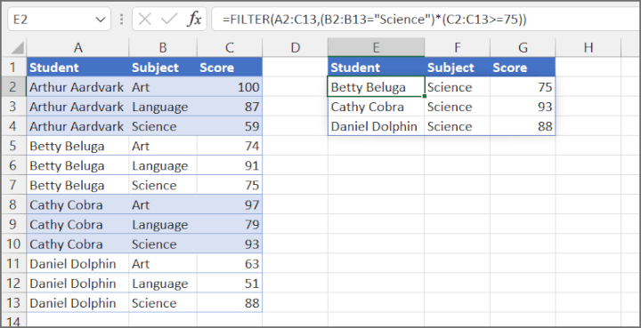

Explanation: The array is the original dataset containing all students’ scores. To isolate scores for Science where students scored 75 or higher, we specify in the include argument that the “Subject” range should be equal to “Science”, add an asterisk (*), and another condition that states the score should be greater than or equal to 75. Note that each condition is enclosed within parentheses.

---

Learn more about other ways of performing a lookup using multiple criteria.

---

Important notes about the FILTER function

• If there aren’t enough empty cells to return all the results, Excel will return a #SPILL! error.
• If array refers to data is in another workbook, that workbook must be open. Otherwise, Excel will return a #REF! error.

5. INDEX/MATCH combo

What does INDEX/MATCH do in Excel?

When used together, the INDEX and MATCH functions perform searches similar to HLOOKUP, VLOOKUP, and XLOOKUP. It is more flexible than VLOOKUP and HLOOKUP, and can be used if XLOOKUP is not available in your version of Excel.

The format of the INDEX/MATCH combo is:

=INDEX(array, MATCH(lookup_value, lookup_array, match_type), column_num)

INDEX/MATCH: What do the arguments mean?

• array is the group of cells containing the lookup and return values.
• lookup_value is the value or the cell containing the value you are searching for.
• lookup_array is the range or array where the lookup values may be found.
• match_type (optional) tells Excel whether to accept an approximate match if an exact match is not found. If this argument is omitted, a match_type of 1 is assumed. 
  • 0 means only exact matches are accepted. Values do not have to be sorted.
  • 1 indicates that Excel should match to the next largest value if an exact match is not found. Lookup_array must be sorted in ascending order.
  • -1 indicates that Excel should match to the next largest value if an exact match is not found. Lookup_array must be sorted in ascending order.

How to use INDEX/MATCH in Excel

A simple example is shown below.

=INDEX(A2:E11,MATCH(B14,C2:C11,0),1)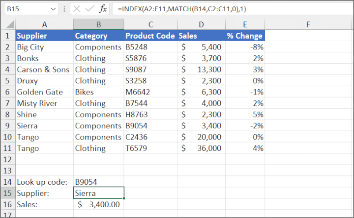

Explanation: The result is that the inner portion of the formula (MATCH) finds that the lookup value is located in the 8th row of the array. The INDEX argument column_num 1 indicates that Excel should return the value in the first column of the array. The value is “Sierra”.

Important notes about using INDEX/MATCH

• XMATCH is the newer version of the MATCH function. XMATCH defaults to an exact match. 
• Wildcard character searches are supported with match_type 0.

6. FIND function

What does FIND do in Excel?

The FIND function performs a case-sensitive search for a specific character or text substring within a cell or text string, and returns the position number of that character, or the start of the substring.

The format of the FIND function is as follows:

=FIND(find_text, within_text, [start_num])

FIND function: What do the arguments mean?

• find_text is the character or substring you want to find.
• within_text is the text in which you want to search.
• start_num (optional) is the position number of the character where you would like to start searching. If omitted, the search begins at the first character of the string.

How to use FIND in Excel

A simple example is shown below. 

=FIND(“feather”,A1)

In this example, we are asking Excel to locate the text “feather” within the values in cell A1. If that text string is found, Excel will display its starting position.

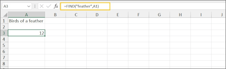In our case, the string making up the find_text argument starts at the 12th character position of the text in cell A1.

Important notes about the FIND Function

1. Since FIND is case-sensitive, if we had entered the formula =FIND(“FEATHER”,A1) above, we would have gotten a #VALUE! error.
2. The optional argument start_num can be useful for skipping known occurrences of text that appear early in the string. For example, =FIND("x","xwx8",2) will return an answer of 3 because we want Excel to ignore the first occurrence of "x" and start searching from the second character in the text string.

7. SEARCH function

What does SEARCH do in Excel?

The SEARCH function searches for a specific character or text substring within a cell or text string, and returns the position number of that character, or the start of the substring. Unlike the FIND function, SEARCH is not case-sensitive.

The format of the SEARCH function is as follows:

=SEARCH(find_text, within_text, [start_num])

SEARCH function: What do the arguments mean?

• find_text is the character or text string you want to find.
• within_text is the text containing the string you want to find.
• start_num (optional) is the position number of the character where you want to start searching. If this argument is omitted, Excel begins searching at the first character in the string.

How to use SEARCH in Excel

A simple example is shown below.

=SEARCH(“FEATHER”,A1)

In this example, we are asking Excel to locate the text “FEATHER” within the values in cell A1. If that text string is found, Excel will display its starting position.

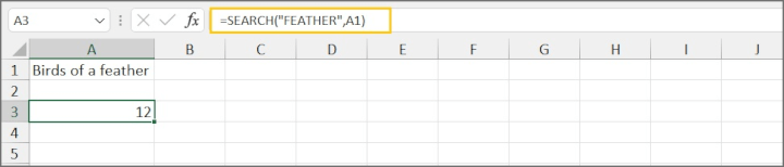Result: The string making up the find_text argument starts at the 12th character position of the text in cell A1. Note that even though our find_text value is in uppercase and the substring in cell A1 is lowercase, it is considered a match.

Important notes about the SEARCH function

1. As mentioned before, SEARCH is not case-sensitive, so it does not matter whether you search in uppercase or lowercase.
2. When using explicit values instead of cell references, find_text must be entered within double quotes.
3. Wildcard character search is supported. This is useful in cases where the exact text string is unknown.

8. LEFT function

What does LEFT do in Excel?

The LEFT function extracts a specific number of characters from a text string, starting from the first (leftmost) character.

The format of the LEFT function is as follows:

=LEFT(text, [num_chars])

LEFT function: What do the arguments mean?

• text is the text string from which you want to extract characters. Text may be entered as a text string within double quotes, or you can use the cell reference that contains the text string you are working with. 
• num_chars (optional) is the number of characters you would like to extract. If num_chars is omitted, the number of characters is assumed to be 1 and LEFT extracts only the leftmost character.

How to use LEFT in Excel

A simple example is shown below. 

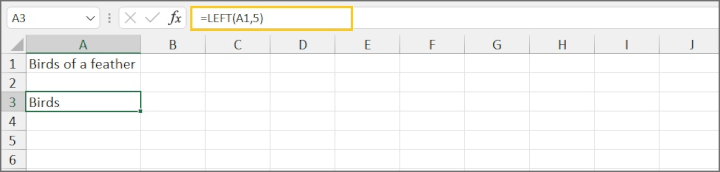
=LEFT(“Birds of a feather”,5)

In this example, we are using explicit text as our text argument, and asking Excel to extract the first 5 characters. The return value is Birds.

The same example using a cell reference is shown below.

Important note about the LEFT function

Consider using TEXTBEFORE if you have Excel 365, as it carries additional features.

9. RIGHT function

What does RIGHT do in Excel?

The RIGHT function extracts a specific number of character(s) from a text string, starting from the rightmost character.

The format of the RIGHT  function is as follows:

=RIGHT(text, [num_chars])

RIGHT function: What do the arguments mean?

• text is the text string from which you want to extract characters. Text may be entered as a text string within double quotes, or you can use the cell reference that contains the text string you are working with. 
• num_chars (optional) is the number of characters you would like to extract, starting with the rightmost character (the one furthest to the right).

How to use RIGHT in Excel

A simple example is shown below.

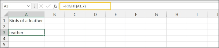
=RIGHT(“Birds of a feather”,7)

In this example, we are using explicit text as our text argument, and asking Excel to extract the last 7 characters. The return value is feather.

The same example using a cell reference is shown below.

Important notes about the RIGHT function

• For advanced use cases of the RIGHT function, check out some more resources here.
• Consider using TEXTAFTER if you have Excel 365, as it carries additional features.

10. MID function

What does MID do in Excel?

The MID function extracts a specific number of characters from a text string, starting at the position you specify. It is usually used when the text you want is bounded on each side by other values.

The format of the MID function is as follows:

=MID(text, start_num, num_chars)

MID function: What do the arguments mean?

• text is the text string from which you want to extract characters. It can either be entered as a text string within double quotes, or you can use the cell reference containing the text you want to work with. 
• start_num is the position number of the first character to be extracted.
• num_chars  is the number of characters to return.

How to use MID in Excel

A simple example is shown below. 

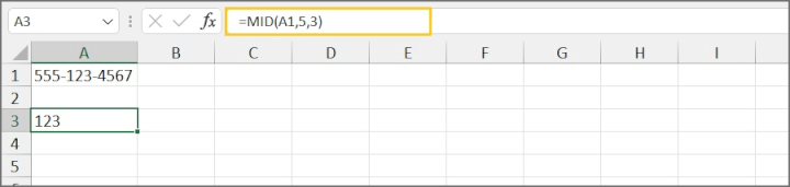
=MID(“555-123-4567”,5,3)

In this example, the text value is entered within double quotes. We have asked Excel to extract 3 characters, starting with the 5th character. The return value is 123.

The same example using a cell reference is shown below.

Important notes about the MID function

• All arguments in the MID function are required.
• For advanced use cases of the MID function, check out some additional resources here.

11. TEXTBEFORE function

What does TEXTBEFORE do in Excel?

The TEXTBEFORE function returns all text that appears to the left of a specific character.

The format of the TEXTBEFORE function is as follows:

=TEXTBEFORE(text, delimiter, [instance_num], [match_mode], [match_end], [if_not_found])

TEXTBEFORE function: What do the arguments mean?

• text is the text string from which you want to extract characters. It can either be entered as a text string within double quotes, or you can use the cell reference containing the text you want to work with. 
• delimiter is a character that marks the “stop” point of the extraction. 
• instance_num (optional) is the nth occurrence of the delimiter. For example, an instance_num of 2 means that Excel should ignore the first occurrence of the delimiter.
• match_mode (optional) is a setting for case-sensitivity. 0 does a case-sensitive search for the delimiter, while 1 is non-case-sensitive. If this argument is omitted, TEXTBEFORE is case-sensitive.
• match_end (optional) treats the end of the text string as the delimiter. This means if match_end is set to TRUE and the instance_num is 1, but the specified delimiter is not found, Excel will return the original text string. If this option is set to TRUE and the instance_num is set to -1, but the specified delimiter is not found, Excel will return an empty string. 
• if_not_found (optional) allows you to return a customized message or value if the specified delimiter is not found. If omitted, the #N/A error message is returned. 

How to use TEXTBEFORE in Excel

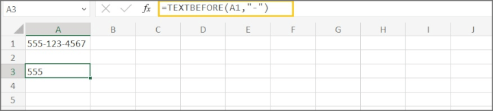
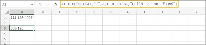
Example 1: TEXTBEFORE with required arguments only

Example 2: TEXTBEFORE with optional arguments

Important notes about the TEXTBEFORE function

• If you use a negative value for the instance_num argument, TEXTBEFORE will search for the delimiter from the end of the text string. 
• TEXTBEFORE is only available in Excel 365 or in Excel for the Web.

12. TEXTAFTER function

What does TEXTAFTER do in Excel?

The TEXTAFTER function returns all text that occurs to the right of a specific character.

The format of the TEXTAFTER function is as follows:

=TEXTAFTER(text, delimiter, [instance_num], [match_mode], [match_end], [if_not_found])

TEXTAFTER function: What do the arguments mean?

• text is the text string from which you want to extract characters. It can either be entered as a text string within double quotes, or you can use the cell reference containing the text you want to work with. 
• delimiter is a character that marks the starting point of the extraction. 
• instance_num (optional) is the nth occurrence of the delimiter. For example, an instance_num of 2 means that Excel should ignore the first occurrence of the delimiter.
• match_mode (optional) is a setting for case-sensitivity. 0 does a case-sensitive search for the delimiter, while 1 is non-case-sensitive. If this argument is omitted, TEXTBEFORE is case-sensitive.
• match_end (optional) treats the end of the text string as the delimiter. This means if this option is set to TRUE and the instance_num is 1, but the specified delimiter is not found, Excel will return an empty string. If this option is set to TRUE and the instance_num is set to -1, but the specified delimiter is not found, Excel will return the original text string. 
• if_not_found (optional) allows you to return a customized message or value if the specified delimiter is not found. If omitted, the #N/A error message is returned. 

How to use TEXTAFTER in Excel

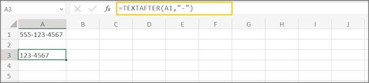
Example 1: TEXTAFTER with required arguments only

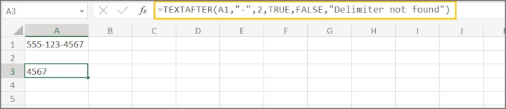
Example 2: TEXTAFTER with optional arguments

Important notes about the TEXTAFTER function

• If you use a negative value for the instance_num argument, TEXTAFTER will search for the delimiter from the text string. 
• TEXTAFTER is only available in Excel 365 or in Excel for the Web.

Ready to become a certified Excel ninja?

Start learning for free with GoSkills courses

Start free trial

Conclusion

Chances are, if you need to look for or extract values in Excel, you will be using one or more of the functions above. Download the free cheat sheet and keep practicing; you’ll be an Excel expert in no time!