Excel Basics - Step by Step Tutorial for Beginners

It’s no secret that Excel is a powerhouse. From database management to complex data visualization and analysis, this dynamic tool isn’t going away anytime soon. 

Most people are so intimidated by Excel that they stay away altogether. But if you’re serious about data management and improving your productivity, you have to start somewhere. We’re here to help you with the basic Excel skills you need to get started. Consider this your very own, starting-from-scratch, Excel tutorial.

The first thing you’ll need to know is what you’re looking at, what it means, and how to find your way around. 

Navigating the interface

One of the most noticeable things about Excel is its gridlike interface. Each rectangle is called a cell, and inside these cells, you can enter information such as text, numbers, and formulas.

Each cell has a unique name, or cell reference, determined by the column and row in which it finds itself.

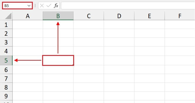
The selected cell above is called cell B5 since it is located in Column B, Row 5. The cell name appears in the Name Box in the upper left corner of the page.

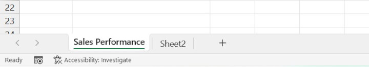
While we’re on the topic, an Excel page is called a worksheet, and the file (or workbook) can have up to 255 worksheets. Worksheets are given the default names Sheet1, Sheet2, and so on, which are shown at the bottom of the screen. But you can rename a worksheet by double-clicking on it and typing the new name right in.

To add a new worksheet, click the plus sign to the right of the last sheet name.

The ribbon

The Excel ribbon appears at the top of the workspace and prominently displays clickable commands that you use to get things done.  Commands are organized by tabs and further divided into command groups.

For example, on the Page Layout tab, you can find the Page Setup command group, where you will see several command options to customize page margins, orientation, size, and so on.

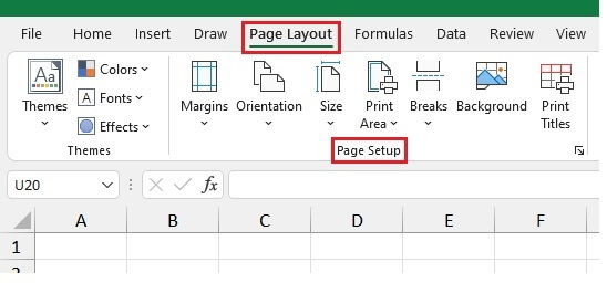
Most commands also have an associated icon that acts as a visual cue and makes Excel friendly to work with. 

The Quick Access Toolbar

Once you settle into using Excel, you’ll probably find that there are commands that you regularly use. Instead of jumping from tab to tab to select those commands, you can store all your favorite commands in one place, known as the Quick Access Toolbar (or QAT).

For example, to add the Sort & Filter command to the QAT, locate that command on the Home tab within the Editing command group.

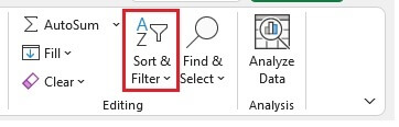
Right-click and select “Add to Quick Access Toolbar” from the contextual menu.

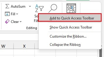
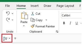
A mini version of the icon will appear on a horizontal pane at the top or bottom of the ribbon.

To remove a command from the QAT, right-click the icon again and select “Remove from Quick Access Toolbar.”

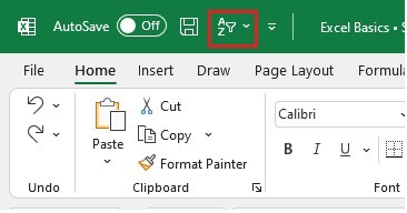
You can change the location of the QAT by right-clicking on a QAT command or anywhere on the QAT pane and selecting “Show Quick Access Toolbar Above the Ribbon.” 

And you can hide the QAT altogether by – you guessed it – right-clicking and selecting “Hide Quick Access Toolbar.” 

Formulas and functions

Now it’s time for the good stuff – using Excel as a productivity tool. There are lots of Excel tools vying for the “Most Useful Feature” trophy, but it’s pretty hard to compete with functions and formulas. Here’s why:

Excel functions and formulas give you over 400 ways to summarize, analyze, and interpret data. They can also help you automate processes and convert data from one format to another. Additionally, formulas are the building blocks to unlocking several other advanced Excel features.

What is a formula?

Any mathematical calculation in Excel is considered a formula. All formulas are basically variations of the four basic operations and are represented as follows:

• + addition 
• - subtraction
• * multiplication
• / division

To let Excel know that we’re looking for the answer to a mathematical problem, the cell input should begin with an equal sign. For example, to find out what is 600 times 99, we would enter:

=600*99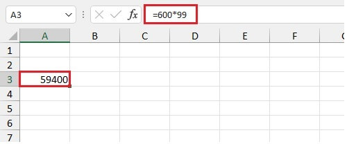

When you press Enter, the result of the formula is displayed in the cell, but the formula you used will be displayed in the Formula Bar.

What is a function?

Functions are a special category of formulas. They can be quite powerful and are built into Excel to perform all kinds of calculations much more quickly and efficiently than basic formulas. 

Here’s a simple example.

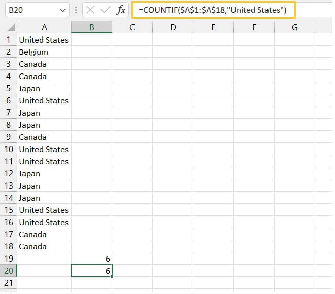
To count the number of times “United States” appears in column A, we could manually enter the number 1 next to each occurrence, then enter a formula to add those numbers.

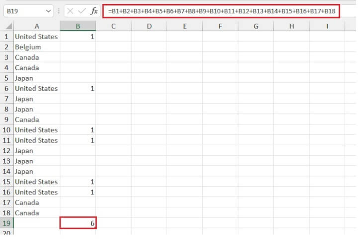
But as you can see, this method is neither time-saving nor reliable. It would be pretty easy to miss one of those occurrences, and frankly, entering those cell references one at a time actually adds to our workload.

A better solution for this task would be Excel’s COUNTIF function. The syntax of the COUNTIF function is COUNTIF(range, criteria). Since functions are still considered formulas, we also start with an equal sign.

=COUNTIF(A1:A18,"United States")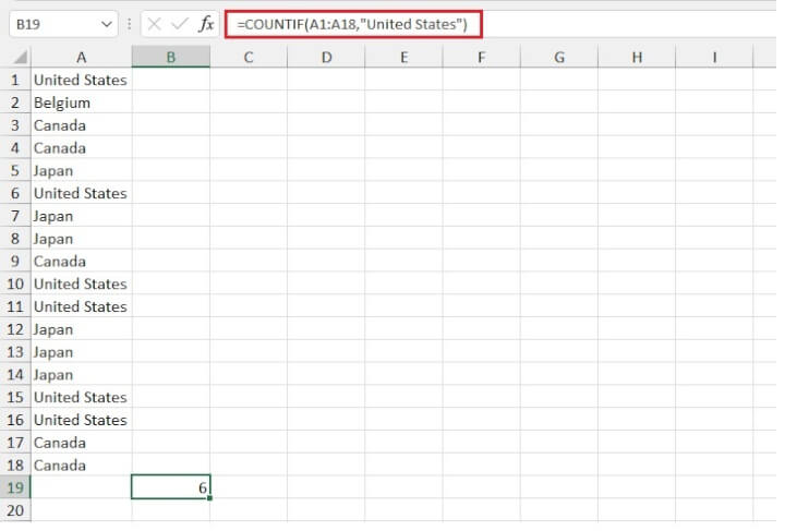

See? It’s easy! Functions are structured as follows:

Equal sign > Built-in function name > Open parenthesis > Arguments in the required format > Close parenthesis

Functions can be entered manually with minimal assistance from Excel, or wizard-style by using the Formulas tab on the Excel ribbon.

Ready to try some functions on your own? We recommend getting started with:

• SUM to add all the numbers in a range of cells

  • =SUM(number1, [number2],...)

• AVERAGE to find the average, or arithmetic mean, of numbers in a range of cells

  • =AVERAGE(number1, [number2],...)

• COUNT to count the number of cells in a range that contain numeric values

  • =COUNT(value1, [value2],...)

For more practice, check out our handy list of twelve essential Excel functions you need to know.

Understanding cell referencing

Now that you know that each cell has a unique name, this next bit of information might throw you for a slight loop. 

When working with Excel formulas, cell references are relative unless stated otherwise. 

Relative cell referencing

Relative? Relative to what? Simply put, relative to the cell in which the formula was entered. This is very important to know, especially when you copy a formula from one cell to another. Otherwise, you may get an incorrect result and not know why, or worse, get an incorrect result without realizing it.

To demonstrate, let’s copy the formula in cell B19 to B20.

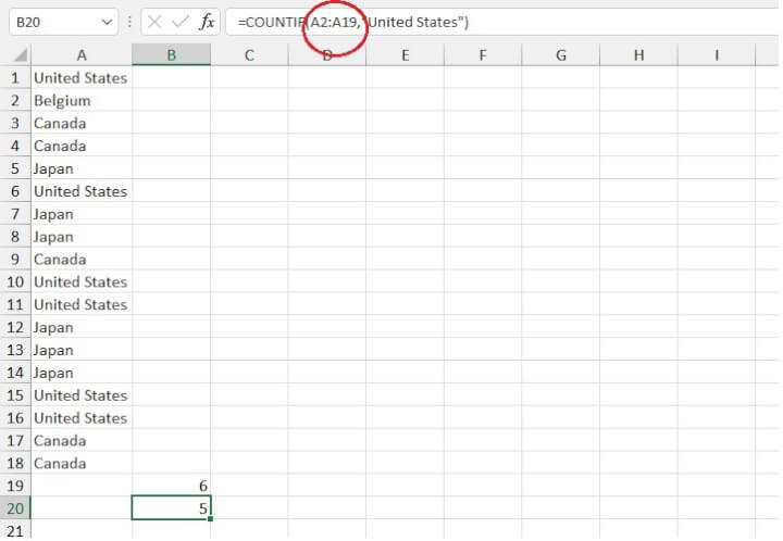
Notice that the structure of the formula stayed the same, but Excel changed the A1:A18 reference to A2:A19, resulting in only five instances of the text in the criteria argument.

We should think of the cell containing the formula as a point of reference, meaning that relative to cell B19, the formula

=COUNTIF(A1:A18,“United States”)

makes reference to a range that is:

• one column left, 
• beginning 18 rows above, and 
• ending one row above

In this case, the range would therefore be cell A1 to A18, but would have been another location if the formula were entered elsewhere. The reason for doing it this way is that it becomes incredibly helpful in situations like the following:

Without relative cell references, we would have to manually enter the cell addresses in column D. Relative cell references make Excel behave smarter when copying formulas whenever we want the same type of action performed. 

Absolute cell referencing

Absolute cell references are the opposite of relative cell references. When a cell reference in a formula is absolute, it means that no matter where that formula is copied to, the reference to that cell remains fixed, or frozen. 

We can make a cell reference absolute by placing a dollar sign before its column name and row number.

=COUNTIF($A$1:$A$18,"United States")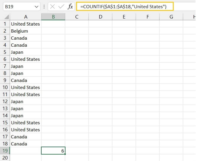

Hot tip: Press F4 (on a Mac, press ⌘+T) right after typing the cell reference to quickly change it from relative to absolute.

 

Now when the formula in cell B19 is copied anywhere, it will search the same range (A1 to A18) for the text “United States”.

Mixed references

A mixed cell reference is one where part of the reference is absolute and the other part is relative. We do this by placing a dollar sign immediately before the fixed element (see below).

• $A1 - reference to column A is fixed; reference to row 1 is relative
• A$1 - reference to column A is relative; reference to row 1 is fixed

Mixed references are typically used when performing matrix-type calculations, such as below.

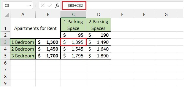
The formula in cell C3 was created with the knowledge that values in column B would be added to values in row 2. However, copying a formula from C3 to C4 would shift the row 2 reference unless we make that fixed. We do this by ‘locking’ or ‘freezing’ that reference with a dollar sign immediately before the row or column which should not shift.

Hot tip: Pressing F4 (on a Mac, ⌘+T) right after typing the cell reference toggles through four possible cell reference structures - absolute, mixed, mixed, and relative.

Managing data

Sometimes the problem with data is that there’s too much of it. When you want to summarize, sort, or temporarily hide some of the information in a data set, Excel has features that you can quickly call up to get the job done.

Cleaning and prepping data

Data management tools like Excel are only as good as the data they’re asked to organize or analyze. If that data is inconsistent or inaccurate, your results won’t be reliable. Data with gaps or inconsistent data types can cause formulas to give an incorrect output, or make functions not perform the way you want them to. So before we start doing anything fancy, we should make sure we have good data.

Identify duplicates

We can easily identify duplicate data by using Conditional Formatting. The steps are as follows:

1. Highlight the data which you suspect may contain duplicates
2. Click Conditional Formatting from the Home tab
3. Click Highlight Cells Rules
4. Click Duplicate Values…
5. In the pop-up window, choose Duplicate under “Format cells that contain:”, and choose the format you would like to apply to the duplicates

Any value that appears more than once in the selected range will have conditional formatting applied.

The above steps are just an indication of where duplicates exist; they don’t actually remove duplicates. When duplicate data means bad data, there are several ways to get you cleaned up.

Remove duplicates

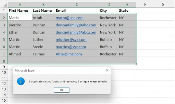
Thankfully, there’s a command right on the Data tab with the name “Remove Duplicates.” This is especially useful for data with multiple columns because you can determine whether a duplicate means all data in that row must be identical to another to be considered a duplicate, or whether only selected columns should be treated as such. We can illustrate this with the example below.

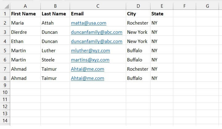
There are no rows that are completely identical to each other, but

• rows 3 and 4 have the same last name, email, city, and state.
• rows 5 and 6 have the same first name, city, and state.
• rows 7 and 8 have the same first name, last name, email, and state.

From a practical point of view, the only real duplicates would probably be rows where the first name, last name, and email address are the same (rows 7 and 8). Maybe Ahmad Taimur moved from one city to another. So we select only those columns and indicate whether our data has headers or not.

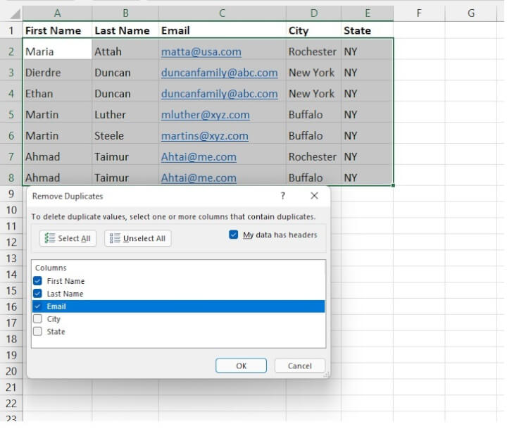
When you click OK, the second occurrence of the duplicate row is deleted.

If you need to preserve the original data, the Remove Duplicates command is not the best method. There are other methods, like advanced filters or Power Query, which do not delete the source data.

Remove blank rows

There are multiple ways to do most things in Excel. Removing blank rows is no exception. The method you choose will depend on your personal preference, the complexity of the data you’re working with, your Excel proficiency, and possibly other factors.

Some favorite methods are:

1. Manually. Yes. If you only have a few rogue blank rows in a relatively small data set, go right ahead: hold down the Ctrl (or ⌘) key, select the blank rows, right-click and delete! 
2. Sorting. Excel’s sorting tool pushes blank rows to the end of the data set. So they basically vanish. If your data is part of an official Excel Table, those blank rows can cause problems later, so be sure to delete the blanks from the bottom of the Table.
3. Filters.  Highlight the data set and click on the Filter icon on the Data tab. Go to the first column header and click the Filter dropdown. Uncheck “Select All” then check “Blanks”. Repeat this process for all column headers. This will leave you with rows that are completely blank. Now, right-click and delete rows. This method works best when there are few columns but several rows.
4. Find & Select. This is a command on the far right of the Home tab. Choose the “Go To Special…” option, and click Blanks and OK. Rows with any blank cell will be highlighted. Right-click any highlighted cell and choose “Delete” > “Delete entire row” from the contextual menu. Note: This method also highlights rows with some blank cells and will potentially delete rows that are partially populated.

Sort data

Sorting data in Excel is all about grouping elements that are like each other. Items can be sorted alphabetically, numerically, in date order, or in some other special hierarchy you have created. Excel can do all of that.

Sort alphabetically

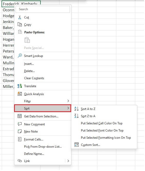
The most frequently used sorting task is probably to put lists in alphabetical order. The quickest way to do this is probably by right-clicking on the data set and selecting the Sort command from the contextual menu.

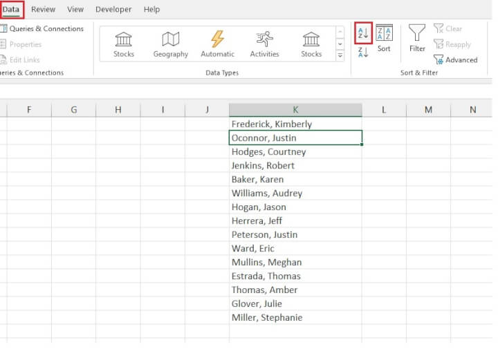
You can also sort by clicking any cell within the data set, then clicking the A-Z sort icon on the Data tab of the ribbon.

And voila! In one click, our list is sorted alphabetically.

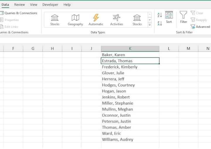
If you wanted the list sorted in reverse order, you would use the Z-A sort icon instead. 

Note that Excel will always treat data in adjacent columns and rows as part of a single data set and sort them together. The opposite is also true. If your data set has blank columns or rows, the Sort feature will separate them and give you a result you may not expect. For cases like this, you should specify the data range to be sorted by manually highlighting that range.

The truth, however, is that most sorting tasks are a little more complicated than our example above. Some data sets have header rows that need to remain in the top row instead of being sorted, sometimes we need to sort or group data by more than one category, and sometimes we want to sort from left to right instead of top to bottom. For all those situations, we would use the Custom Sort icon.

Custom Sort

When you want to have a bit more control over how Excel sorts your data, use the Custom Sort icon (right next to A-Z and Z-A). The Custom Sort command does the following:

1. highlights the area it intends to work with
2. shows a dialog box where you can check or uncheck whether the highlighted area carries row headers
3. allows you to add additional options, like 
   • sort using multiple levels
   • sort from left to right
   • sort by color
   • case-sensitive sorting, and more

Below is a data set that lends itself to multi-level sorting.

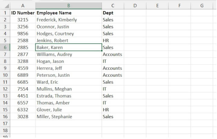
To sort by department name and then alphabetically within each department, follow these steps:

1. Click anywhere within the data set
2. Select the Custom Sort icon
3. Row 1 is a header, so it should not be sorted with the rest of data (the “My data has headers” box should be checked)
4. Sort by Dept column, Sort on Cell Values, in A to Z order
5. Click Add Level
6. Go to the “Then by” row, select Employee Name from the first dropdown. The other options should say Cell Values and A to Z.

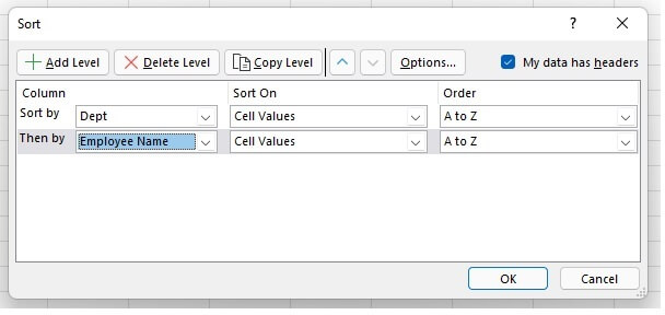
7. Click OK

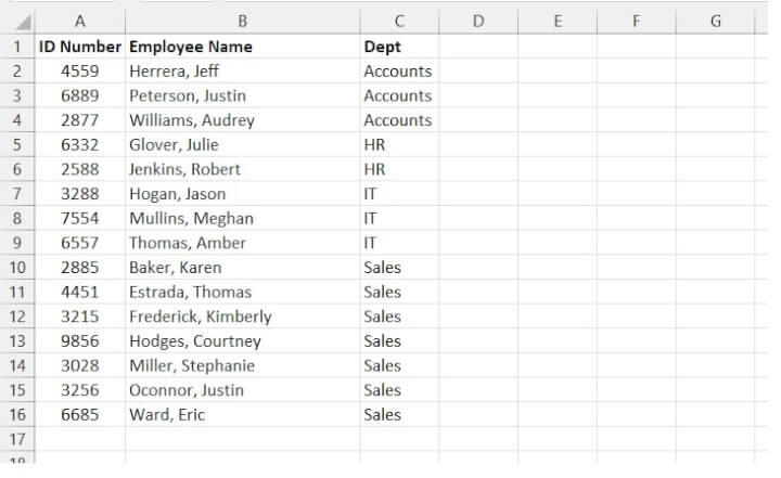
The finished product will look like this:

Troubleshooting

Did you run into any problems while sorting? We’ve got you covered. Some of the most common reasons for unexpected results while sorting are:

• Hidden rows or columns
• Data inconsistency
• Multi-row headers

Filter data

If you ever want to temporarily hide some rows of data based on certain criteria without deleting them, applying an Excel filter is probably your best option. 

Auto-filters

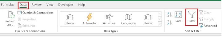
Auto-filters are easy to use, flexible and super-handy. The Auto-filter command is located on the Data tab of the ribbon, but you can also access it from the Home tab by clicking on the Sort & Filter dropdown command.

Excel allows you to filter by:

• Matching values
• Partial matches
• Rows that contain or do not contain certain values
• Color
• Wildcard characters using the “Custom Filter” option

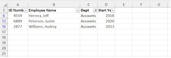
In the dataset below, a simple filter can be applied to display only the records of employees from the Accounts Department.

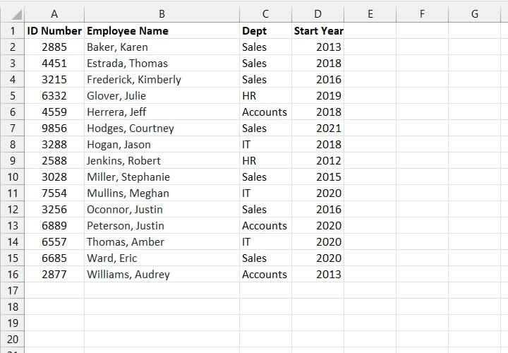
1. Click a cell within the dataset, and select the Filter command
2. Click the filter arrow in the Dept column
3. Uncheck the Select All checkbox
4. Check the “Accounts” category and click OK

All rows outside of that category will be hidden.

To redisplay all the rows in the dataset, click the column which shows a filter funnel and reselect all, or deselect the Filter command on the ribbon.

Advanced filters

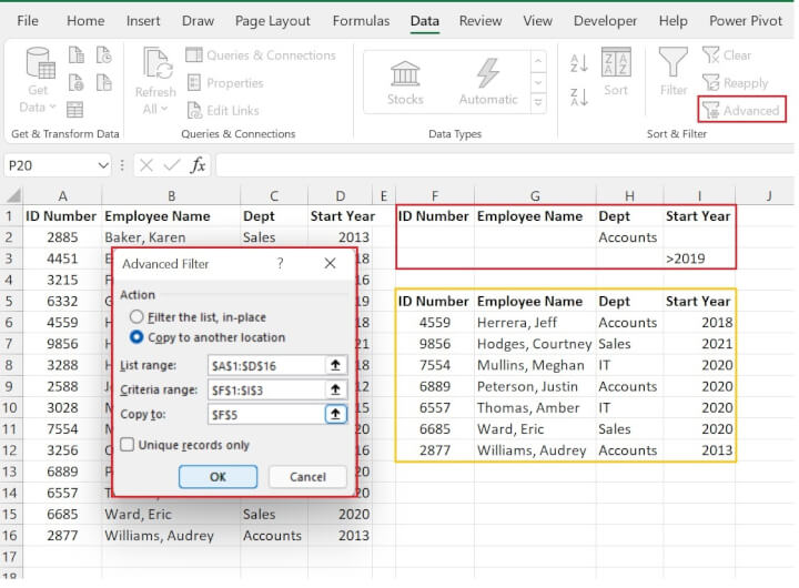
While Auto-filters allow OR logic using a single column with its Custom Filter option, advanced filters allow OR logic using up to two columns. For example, we can view all employees from the Accounts department and all employees who joined after the year 2019 by using the Advanced filter feature –  something an auto filter cannot do.

Learning how to use the advanced filter command in Excel is sure to put you a step ahead since it is an often-forgotten feature.

1. Go to the Data tab and click the Advanced filter icon.
2. You can choose to either filter the list in place, or copy to another location within the same worksheet).
3. For the ‘List Range’ field, select the list to be filtered, including column headers.
4. Select the criteria range which includes the header name(s) and the value(s) which will be used to apply the filter (e.g. F1 to I3 in the above example).
5. If ‘Copy to another location’ was selected, click on the cell where you want the filtered list to appear in the ‘Copy to’ field.
6. Click OK.

Cell formatting

Accurate data is and should be a high priority for obvious reasons, but making data visually appealing is also an important step in how we analyze that data and make decisions. A spreadsheet that is difficult to read or where the meaning of the values is unclear is a turn-off and might make hours of hard work pointless. 

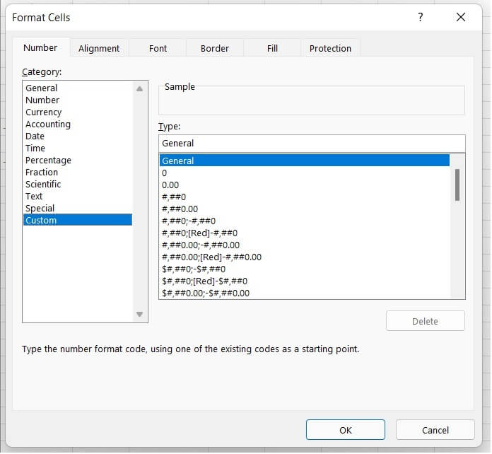
The Format Cells dialog box can be considered ground zero for any type of cell formatting. You can right-click on a cell and select Format Cells from the context menu. More often though, you’ll likely be using the Ctrl+1 (⌘+1 on Mac) shortcut.

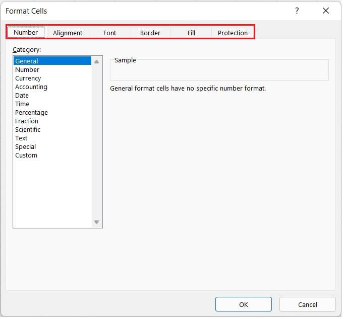
Below are a few common options for formatting cells.

Number formats

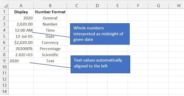
A number format can influence the number of decimal places in a number, the way a date is displayed, currency symbols, and so on. By formatting numbers in Excel, we do not change the value of the number – we simply change the way it appears.

In the example below, the value “2020” was entered into each cell from A2 to A9 with a different number format applied. 

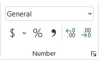
You can also use the Number command group on the Home tab to get more number formatting options.

Currency vs. Accounting format

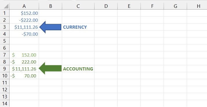
The Accounting and Currency formats are quite similar, the main difference being that in Accounting, currency symbols are left-aligned, and decimal points line up with each other. With the Currency format, values are right-aligned.

Custom number formats

If none of the built-in formats suit your needs, you can even create your own custom number format by using format codes from the Custom category.

Cell alignment

Text values in Excel are left-aligned by default, and numeric values are right-aligned by default. However, you can manually change these at any time by selecting the cell(s) you want to change and clicking one of the options in the Alignment command group. 

The Alignment tab in the Format Cells dialog box carries several detailed options to control text direction, orientation, and indentation.

Merge two or more cells

If the value in a cell is spread across several columns and you want to make it more presentable, you can merge the affected cells to behave like a single cell. You can either use:

1. Merge & Center, or
2. Center Across Selection

Merge & Center

This method is often used because it has a dedicated command right on the Home tab, so it’s easily executed.

Just highlight the cells that should be merged, click Merge & Center, and it’s done!

Drawbacks when using Merge & Center

1. This command only preserves data in the first (top-left) cell of the highlighted range. Any data in the other cells will be deleted.
2. Selecting cells of different sizes can be problematic.
3. Sorting can be problematic since sorted cells must be of the same size.

For the above reasons, the Center Across Selection option is preferred by most Excel experts.

Center Across Selection

To use Center Across Selection:

• Select the relevant cells.
• Press Control + 1 or right-click and choose Format Cells from the menu.
• In the Alignment tab, from the Horizontal drop-down, select Center Across Selection.
• Click OK

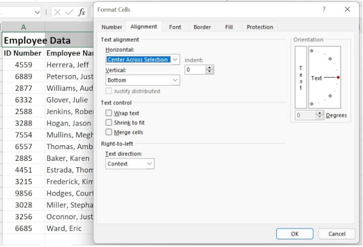
Text will appear merged and centered, but each cell can still be selected individually. They can also be sorted and highlighted as normal.

If data is in any cell other than the top-left cell, there will be no loss of data.

Conditional formatting

Conditional formatting dynamically changes the way text, numbers, or cells appear based on a certain condition being met or not being met. It’s a very effective way to help you understand patterns you might have missed otherwise.

Conditional formatting commands can be accessed from the Home tab in the Styles command group.

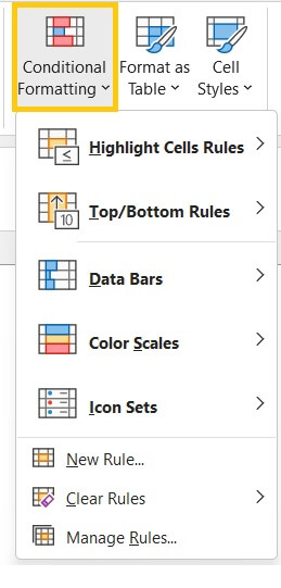
You can use the built-in rule templates (Highlight Cells or Top/Bottom) to identify the cells to be specially formatted, or you can create your own rule from scratch using the New Rule option.

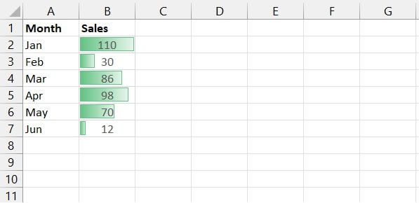
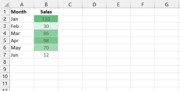
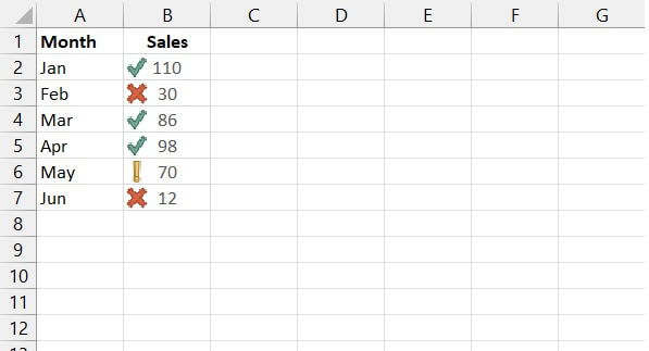
Data Bars, Color Scales, and Icon Sets

With Data Bars, you can mimic Excel bar charts and use color to show how quantities within a range compare with each other.

With Color Scales, you can use a color’s intensity to depict the same thing.

Icon Sets use a combination of shapes and colors to convey whether a value should be considered negative or positive.

The best part of conditional formatting is that it is dynamic, so when the data changes, Excel uses the rule(s) you created to determine whether the conditions are still met, and will update the formatting automatically.

Other formatting changes

Cosmetic changes such as font size and style, strikethrough effect, cell borders, etc., can be accomplished from the Home tab or the respective tab in the Format Cells dialog box.

Control your view

Excel allows you to enter and store lots of data, but that doesn’t mean you always want to see it all at once. 

Freeze panes

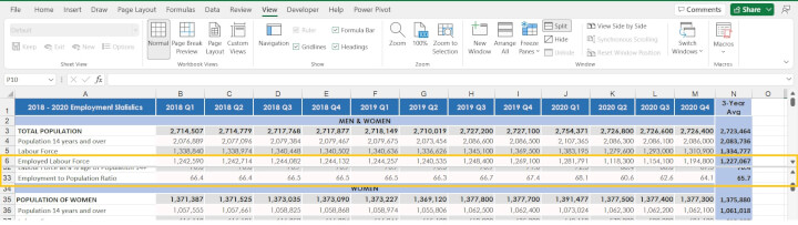
For example, on a very large spreadsheet, you might find it very difficult to manage your data or even know what you are looking at because header rows or important columns are no longer visible when you scroll through the data set.

On the View tab, the Freeze Panes command lets you “lock” certain rows or columns so that they are always in view, no matter how far away you scroll.

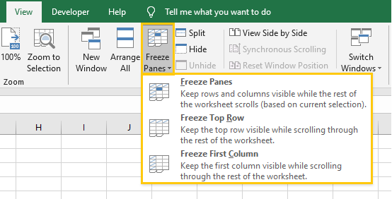
There are three options available:

1. Freeze Panes - visible rows and columns above the active cell will be frozen
2. Freeze Top Row - the first visible row will be frozen
3. Freeze First Column - the first visible column will be frozen

To unfreeze, return to the Freeze Panes dropdown, and ‘Unfreeze Panes’ will be the first command if any rows on the active worksheet were frozen.

Split worksheet view

Another option for controlling your view is to split the panes so that you can see separate sections of the worksheet at once with the Split command. When the ‘Split’ command is activated, you can divide the window into different panes that scroll separately.

The Split command is located next to Freeze Panes on the View tab. You can apply a vertical, horizontal, or four-way split, depending on the location of your active cell. The window you click on will become the active one, allowing you to scroll while keeping the inactive window(s) fixed.

Excel with Excel

Remember, just because you can add every color of the rainbow to your worksheet doesn’t mean you should. Generally speaking, it’s better for your presentation to be understated than overdone. We’ve put together some best practices for Excel presentations, and free templates for money management, personal projects, business planning, and project management.

Now that you’ve learned enough to get started, you should probably know that there are shortcuts to do practically everything in Excel. Check out our cheat sheet of Excel hacks to organize and analyze data like a pro.

Want to work on some of these skills we just shared? Practice with this free one-hour crash course and downloadable exercises!

Even better, start learning more formulas, functions, and time-saving hacks today with the Microsoft Excel - Basic course.

 

Ready to become a certified Excel ninja?

Start learning for free with GoSkills courses

Start free trial